RNA 3D Structure Course
by Craig L. Zirbel and Neocles Leontis at Bowling Green State University
Link to this document: https://tinyurl.com/RNA3DStructureCourse
This material was first developed by Craig L. Zirbel while visiting the University of Vienna and teaching a course in the Institute for Theoretical Biology in 2013-2014. Additional material was added by Professor Leontis in many places, especially when this material was used for workshops at the Rustbelt RNA Meeting. There are many exercises which we suggest that you take the time to do.
Table of contents (should also be available in the left side bar)
Online Recorded Lectures and Slides by Professor Leontis on RNA from 2013
Software for visualizing 3D Structures in PDB format
The RNA Bases: Purines and Pyrimidines
Exercise 1: Get to know the RNA bases
RNA base hydrogen bonding potential
Exercise 2: Canonical Watson-Crick AU and GC base pairs
Leontis-Westhof system for annotating RNA basepairs
Basepair orientations cis and trans
Three-character annotation of RNA basepairs
Exercise 3: Canonical Watson-Crick basepairs
Exercise 4: Triangle representation of RNA basepairs
Exercise 5: Annotating RNA basepairs
Exercise 6: Annotate successive RNA basepairs
Exercise 7: Form potential RNA basepairs from hydrogen bonding potential
Exercise 8: Annotate RNA basepairs
Symbolic representation of base pairing
Leontis-Westhof basepair symbols
Exercise 9: Using Leontis-Westhof symbols
Exercise 9: Identify 3’ and 5’ faces of bases
Exercise 10: Annotate base stacking
Exercise 11: Annotate base stacking
Symbols for base stacking from François Major’s group
Suggestions for making 2-dimensional RNA interaction diagrams
Exercise 13: Annotating an RNA motif
Base-phosphate interaction locations
Base-phosphate interaction and the assignment of atoms to nucleotides
Base-phosphate interaction character annotation
Base-phosphate interaction symbolic annotation
Exercise 14: Annotate base-phosphate interactions
Exercise 15: Annotate base-phosphate interactions in a helix
Exercise 16: Annotate base-phosphate interactions in a motif
Exercise 17: Extended investigation of basepairs
Anti versus syn conformation of the glycosidic bond
Exercise 18: Anti and syn in RNA helices
Exercise 19: Annotate anti and syn conformation
Exercise 20: Annotate anti and syn in an RNA motif
Exercise 21: Annotate anti and syn in an RNA motif
Experimentally determined RNA 3D structures
Where can one get RNA 3D structures?
Tour of RNA 3D structures using Representative Sets
Sequence variability in structured RNA molecules
Nucleotide to nucleotide alignments of RNA 3D structures
Exercise 22 - needs to be rewritten
Choosing basepair exemplars from each basepairing family
Displaying basepair exemplars from each geometric basepairing family
Position of glycosidic bonds in RNA basepairs in the same geometric family
IsoDiscrepancy Index to measure the degree of isostericity between two basepairs
IsoDiscrepancy values within each geometric basepairing family
Interactive RNA secondary structure
Exercise 25: Analysis of a tRNA structure
Sequence variability in the Sarcin-Ricin motif
RNA 3D Motif Atlas entry for instance IL_1S72_103 of the sarcin-ricin loop
RNA 3D Motif Atlas motif group IL_49493
Multiple sequence alignments of RNA sequences
Sequence variants of instance IL_3V2F_007 of the sarcin-ricin internal loop
Sequence variants of the sarcin-ricin motif across many instances
Inferring the geometry of RNA motifs with JAR3D
Searching RNA 3D structures with FR3D
Other interactions on circular diagrams
Symbolic search for two basepaired nucleotides
Exercise: Search for all GA basepairs in which G uses its Sugar edge
Exercise: Motif diagram for the core of the Sarcin-Ricin loop
FR3D symbolic constraint summary
Nucleotides which border or delimit a single-stranded region
Exercise: Symbolic search for hairpin loops and a little bit of context
Exercise: Symbolic search for internal loops
FR3D geometric and mixed searches
GNRA hairpin loop geometric search
FR3D guaranteed results in geometric searches
What determines the 3D structure of a 3-way junction?
Internal loop sequences with different geometry
Getting and using the Swiss PDB Viewer Program: Short Presentation
Goals of the Rustbelt Workshop
RNA resources
Online Recorded Lectures and Slides by Professor Leontis on RNA from 2013
Databases for RNA Structure
- PDB: Protein Data Bank
- PDB101
- NDB: Nucleic Acid Database
- RNA Basepair Catalog
- BGSU RNA representative sets and equivalence classes
- BGSU RNA structure atlas
Software for visualizing 3D Structures in PDB format
- SwissPDBViewer Full Tutorial
- SwissPDBViewer Download Link and SwissPDBViewer: A Short Tutorial Video
- Pymol Tutorial: https://bioquest.org/nimbios2010/wp-content/blogs.dir/files/2010/07/pymol_tutorial3.pdf
- Chimera Tutorial: https://www.cgl.ucsf.edu/chimera/tutorials.html
What is RNA?
RNA compared to DNA
Like DNA, RNA is a linear polymer made from repeating units called Nucleotides. Like DNA, RNA has four nucleotides (A, G, C, and U instead of T in DNA). RNA is usually single-stranded while DNA is usually double stranded, with two complementary strands forming long Watson-Crick base-paired double helices.
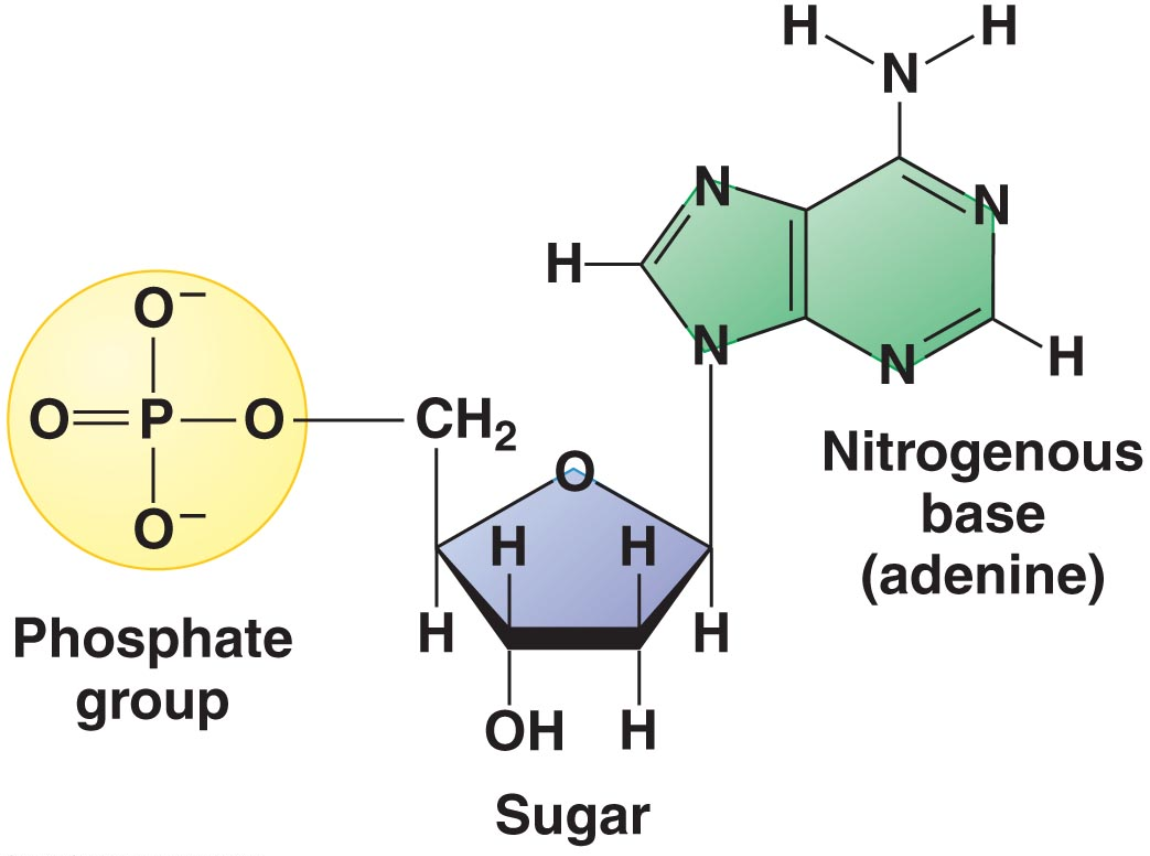
What is a nucleotide? Each RNA or DNA nucleotide is made of three parts: A base (A, C, G, and T or U), a sugar (ribose or deoxyribose), and a phosphate group, connected covalently.
RNA nucleotides vs. DNA nucleotides: Both RNA and DNA nucleotides consists of three parts: A planar, Aromatic Base (consisting of C, N, O and H atoms), a sugar ring, and a negatively charged phosphate group (PO4). There are four types of bases in DNA (A, C, T, and G) and four in RNA (A, C, U, and G). There are two differences between DNA and RNA nucleotides:
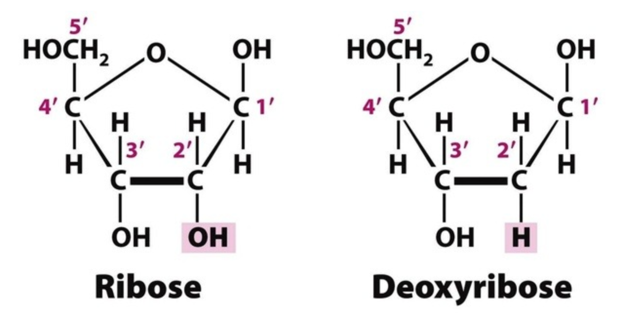
- The sugar in RNA is Ribose and the sugar in DNA is 2’-deoxy-ribose. This just means that in DNA, the 2’-OH in RNA is replaced by -H as shown:
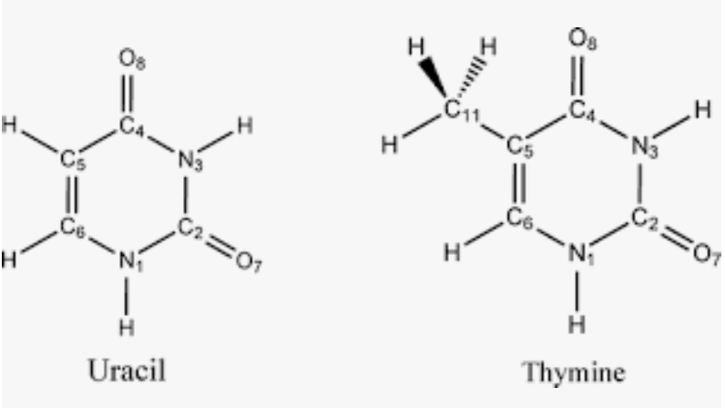
- The Thymine base in DNA replaces Uracil in RNA. Thymine is just Uracil with a -CH3 (methyl) group at position 5 of the base in place -H.
Why does DNA have T? One of the most common forms of DNA damage is hydrolytic deamination of C to form U, which can pair with G to form a “wobble” pair. To repair such damage before it can lead to mutations, cells have an enzyme called uracil-DNA glycosylases that detect U in DNA and cut it out. Other enzymes replace the damage and restore C opposite G. Because in DNA T is found opposite A in place of U, the cell can detect where C is supposed to go during the repair process, because uracyl-DNA glycosylase only removes U and T.
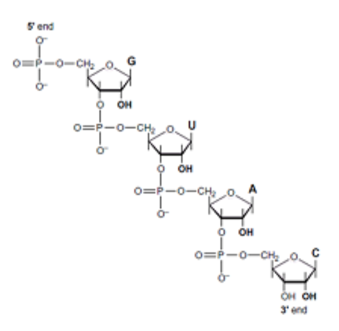
How are nucleotides linked? DNA and RNA nucleotides are linked to each other by covalent phospho-ester bonds. Each phosphate links the two sugars of neighboring nucleotides together as shown →. The phosphates form phospho-ester bonds with the hydroxyl groups at the 3’- and 5’-positions of neighboring sugar units. The Base is attached to the C1’ position. The ring Oxygen is the 4’-O-.
DNA is double stranded and RNA is single stranded:
DNA is usually double-helical, due to the way it is replicated, comprising two complementary molecules running anti-parallel to each other. In DNA, each base is opposite its complementary base on the other strand (A opposite T and G opposite C), forming canonical Watson-Crick AT and GC base-pairs, that stack on each other like plates to make B-form, anti-parallel double helices.
RNA is usually single-stranded. But, by folding back on themselves, RNA molecules generally form short complementary double helices composed of AU and GC Watson-Crick basepairs, with occasional GU base-pairs (“wobble” pairs).
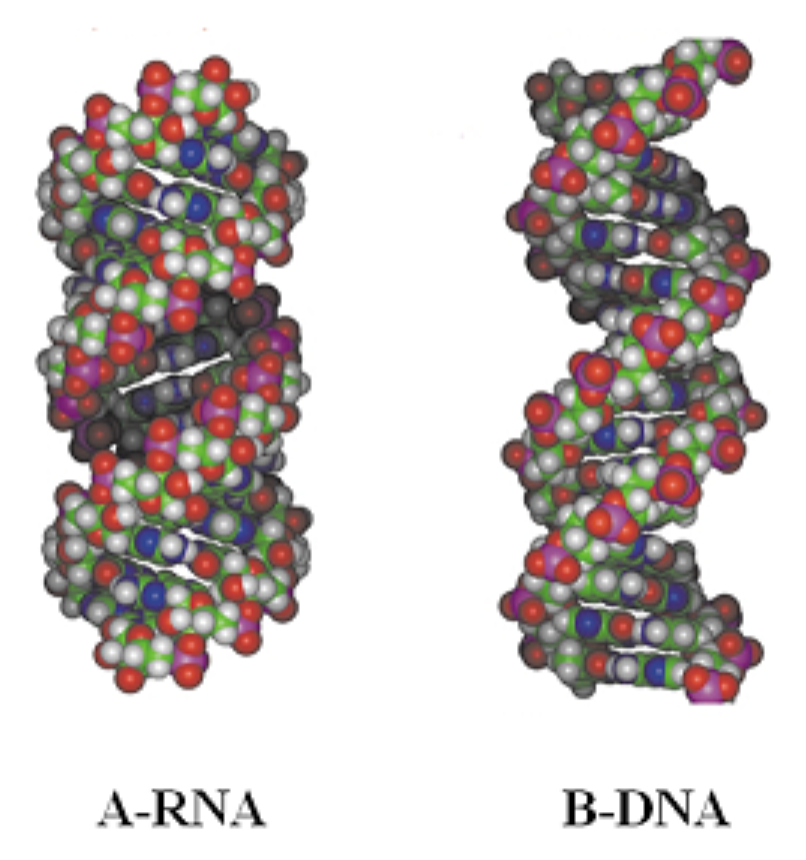
DNA helices are usually B-form while RNA helices are always A-form. Both are Right-handed.
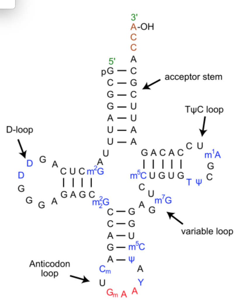
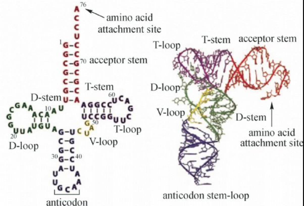
What is secondary structure? The Watson-Crick-paired helices of RNA molecules correspond to the “secondary structure,” which is usually used to depict the structure of RNA molecules in a planar, easy-to-read format. As an example, this is the secondary structure of a tRNA, which consists of four helical regions (the “acceptor stem” to which the amino acid is attached to the 3’-OH), the D-stem, the anti-codon stem and the T-stem. tRNAs have 3 hairpin loops and one four-way junction (4WJ). The anti-codon loop has three nucleotides (in red) complementary to the corresponding mRNA codon for the amino acid. tRNA generally have several modified bases, shown in blue.
The RNA Bases: Purines and Pyrimidines
There are two types of bases in RNA and DNA, purines (A and G), consisting of fused 5 and 6 member rings, and Pyrimidines (A and U or T), consisting of 6 member rings. The purines, A and G, have the same ring atoms and only differ as to the attached (“exo-cyclic”) groups, which can be -NH2 or =O. The same applies to the pyrimidines, U and C. See Figure 1 below.
In the first several visualizations below, hydrogen atoms are shown, but in later visualizations, hydrogen atoms are not always shown.
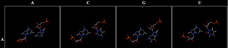
Exercise 1: Get to know the RNA bases
Open the 3D views of RNA bases A, C, G, and U at this link.
- Model selection: Use the checkboxes to view one RNA nucleotide at a time. When colored by base, A is red, C is yellow, G is green, U is blue. This is the default coloring.
- Coloring: Change the coloring to “CPK” to view individual atoms using the “Coloring Options” feature. In CPK coloring Oxygen is red, Nitrogen is blue, Carbon is gray, Hydrogen is white and Phosphorus is orange.
- Rotation and Panning: Click and drag in the viewing box to rotate. Double click and drag to pan side to side. (On a PC, Control Right click to pan.)
- Zooming: You may be able to zoom in and out by rolling the mouse wheel. If not, press shift and click, then move the mouse forward and back to zoom in and out, or side to side to rotate.
- Atom ID: Hover over an atom to see what atom it is. The format is: [base]nucleotide number:chain.atom name atom number.
- Measure Distances: You can measure distances between atoms by double clicking the first atom and then double clicking the second atom. What is the distance between the N1 and C2 atoms in the U base? Give the answer to three decimal places in nanometers (nm).
- Measure Bond Angles: You can measure angles by double clicking the first atom, clicking the second, and double clicking the third atom.
Hydrogen Bonds vs. Covalent Bonds
Covalent bonds are much stronger (~400 kJ/mole) than the Hydrogen-bonds (H-bonds) that hold RNA base-pairs together (15-25 kJ/mole), so covalent bonds are more permanent, while H-bonds and other non-covalent interactions form and break readily during biological transformations.
RNA base hydrogen bonding potential
Around the outside of an RNA base one finds chemical groups that have polar bonds, allowing them to form H-bonds. The atoms forming polar bonds, N, O, and H, have partial electrical charges. The partial charges are made apparent in the images below by coloring. Full-resolution versions of these images were published in this review chapter by Sweeney, Roy, and Leontis (2015). The following text was adapted from that article:
How to recognize H-Bond Acceptors:
For each base, the hydrogen bond acceptor groups are colored red, to reflect their partial negative charge. H-bond acceptor groups in RNA are “Localized Lone Pairs of Electrons on Oxygen or Nitrogen Atoms.”
Note: Lone pairs that are Delocalized and involved in Pi-bonding of the aromatic ring systems are NOT Hydrogen-bond Acceptors. For example, the lone pairs of exocyclic -NH2 groups on A, C, and G bases are delocalized, so the -NH2 groups only act as H-bond Donors.
How to recognize H-Bond Donors:
H-bond donor groups are comprised of hydrogen atoms covalently bonded to electronegative oxygen or nitrogen atoms. They are colored blue, reflecting their overall positive charges. The 2’-OH (hydroxyl) groups are colored purple to indicate that they can serve either as Hydrogen-bond donors or acceptors (or usually BOTH at the same time) and can therefore interact with two groups simultaneously. Each hydroxyl Oxygen atom has two localized electron lone pairs that act as acceptors. The H-atoms bonded to Nitrogen are in dark blue indicating they have more positive charge than the H’s attached to carbon atoms (shown in light blue). The darger blue indicates H-bond donor groups that make stronger H-bonds.
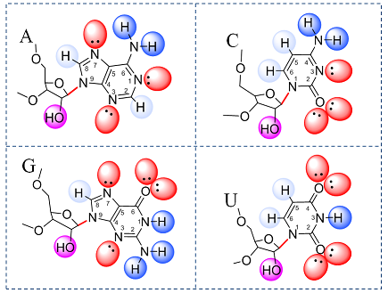
Figure 1. RNA base hydrogen bonding groups. H-bond donors in blue and H-bond acceptors in red.
RNA base pairs
RNA bases are often observed to lie in the same plane and to make hydrogen bond interactions with one another. These are called RNA base pairs. They are found in a rather small number of different geometries, dictated by the locations of positively and negatively charged regions around the sides of the bases.
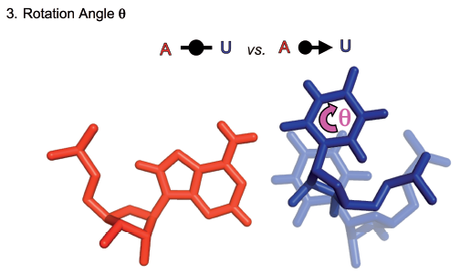
Exercise 2: Canonical Watson-Crick AU and GC base pairs
Roughly ⅔ of the base pairs in an RNA molecule are what are called “canonical” Watson-Crick AU and GC base pairs. These are the analogue of the Watson-Crick basepairs in DNA. Please familiarize yourself with these basepairs at this link. The first two instances are from a very high resolution structure (0.9 Angstrom resolution) which shows the hydrogens, the next two are from a high resolution structure (2.4 Angstroms) which does not show the hydrogens, and the fifth instance is a long RNA double helix. It’s good to be able to recognize the bases and their edges both with and without the hydrogens.
- Color instance 1 with CPK coloring. Write down the G atoms that are making apparent hydrogen bonds with C atoms and write down the bond length (double click interacting atoms to find the length). The center one is G-H1 with C-N3, bond length 0.214 nm. Now write down the others.
- Color instance 2 with CPK coloring and list the apparent hydrogen bonds and their lengths. One is significantly longer than the other two, and so is not as strong.
- The atoms of one base that make hydrogen bonds with the atoms of the other base form the “Watson-Crick” edge of each base.
- Instances 3 and 4 are typical of most RNA 3D structures which do not have hydrogens shown. Get familiar with these as well, and learn to identify the Watson-Crick edge. If you select both instances 1 and 3, you can see the two pairs superimposed. Click next to see instances 2 and 4 superimposed.
- The glycosidic bond connects each base to its ribose sugar by a covalent bond. Make note of the RNA base atom on one end of the glycosidic bond (N1 or N9) and the sugar atom on the other end of the glycosidic bond.
- The ribose sugar is a non-planar 5-sided ring that includes one oxygen. Note the numbering of the ribose atoms in the diagram below.
- From there, the nucleotide connects to the phosphate group, which looks like a Y at the end of each nucleotide. When joined to another nucleotide, each phosphorus atom (P) will have four oxygen atoms attached to it. Write down the names of the oxygen atoms connected to the phosphorus atom.
- Click View Neighborhood to see nearby nucleotides. Find the fourth oxygen connected to the phosphorus atom of one of the original colored bases, and note the name of this oxygen atom and where it connects to the next nucleotide. Note: bonds between gray and colored bases are not shown in the viewing window.
- Instance 5 shows a long double helix made by stacked canonical Watson-Crick basepairs. Using default coloring, check to see that all are GC or AU. On a PC, Control-Right-Click can be used to pan the coordinate viewer, which helps to see the two ends of the double helix. Viewed from the end, you can see how perfectly regular the double helix is.
- How many basepairs are needed to make a complete turn of the double helix? Call that number N. That is, the double helix repeats every N basepairs.
- Go to this google slide presentation of RNA bases, create a new page, add your name, and pick two RNA bases and rotate and/or flip them to match red with blue and so make different RNA basepairs.
Non-Watson-Crick basepairs
When RNA chains fold back on themselves, one often sees short stretches of complementary bases which make Watson-Crick GC and AU basepairs. If that is all that RNA did, it would be very similar to DNA. But the strands of RNA come together in many different ways, and the bases come together in planar, edge-to-edge hydrogen bonding interactions in many different conformations than Watson-Crick basepairs. These are key to understanding RNA 3D structures and their sequence variability between different organisms.
Leontis-Westhof system for annotating RNA basepairs
We now introduce a standard way to refer to the different types of basepairs that RNA bases can make. It is a simple system devised by Neocles Leontis and Eric Westhof and originally appeared in the 2001 paper “Geometric nomenclature and classification of RNA base pairs” which is available at this link. Soon after, a paper by Leontis, Stombaugh, and Westhof showed the best known examples of each RNA basepair, see “The non‐Watson–Crick base pairs and their associated isostericity matrices” from 2002 at this link.
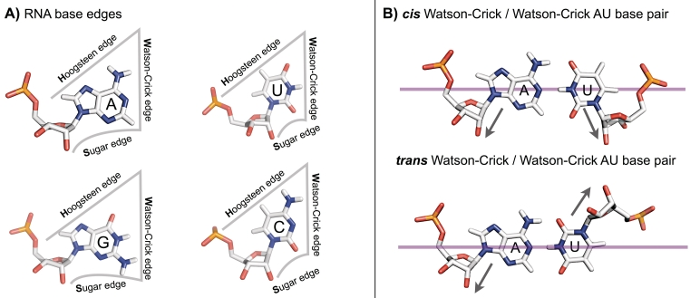
Figure 2. Leontis-Westhof system for base edges and basepair orientation. From Comprehensive survey and geometric classification of base triples in RNA structures, by Amal S. Abu Almakarem, Anton I. Petrov, Jesse Stombaugh, Craig L. Zirbel, Neocles B. Leontis, 2011, available at this link.
Base edges
In their 2001 paper, Leontis and Westhof divided the outside atoms of each RNA base into three edges, called Watson-Crick, Hoogsteen, and Sugar Edge. These are shown in the left panel of Figure 2. Note that the sugar edge includes the 2’-OH group attached to the ribose sugar ring. Note that in Figures 1 and 2, the Watson-Crick edge of each base is on the right side of the base. When two RNA bases meet in the same plane, one can usually describe the basepair that is being made by telling which edge of each base is making the contact. This system is descriptive enough to capture nearly all recurring RNA basepairs, without being overly detailed. As you look at examples, keep in mind that the Leontis-Westhof system chooses a certain balance between simplicity and detail. In some cases, more detail might be warranted.
Basepair orientations cis and trans
In the top of the right panel of Figure 2, one sees a C (on the left) using its Watson-Crick edge in a basepair with a G (on the right). This is the most common RNA basepair, which occurs in RNA helices. In the bottom of the right panel, one sees a U (on the left) using its Watson-Crick edge in a basepair with the Watson-Crick edge of an A. But this is not the common UA basepair from RNA helices. The bases are not in the right orientation for that; in order to make that basepair, one would need to flip one of the bases 180 degrees out of the plane before bringing the Watson-Crick edges together again. The possible orientations of the bases can be distinguished by noting whether the glycosidic bond, which connects the base to the ribose sugar of the backbone (overlaid with dark arrows in the figure) both lie on the same side of a line through the two bases (called cis) or on opposite sides of the line (called trans). The top basepair is in cis, the bottom one in trans. The basepairs in RNA helices are cis Watson-Crick / Watson-Crick basepairs. The 2001 Leontis-Westhof paper simply says about cis and trans that they “follow the usual stereochemical meanings” which you can read about in a Wikipedia article at this link. In particular, it says there that “The terms cis and trans are from Latin, in which cis means "on the same side" and trans means "on the other side" or "across".”
Three-character annotation of RNA basepairs
The Leontis-Westhof system allows for a simple 3-character description of each RNA basepair, using c or t for cis or trans, and W, H, or S for each of the interacting edges. Thus, for example, the top basepair in Figure 2 is annotated AU cWW for a basepair made between A and U in which A uses its Watson-Crick edge, U uses its Watson-Crick edge, and the basepair orientation is cis. The bottom basepair is annotated AU tWW.
Exercise 3: Canonical Watson-Crick basepairs
Revisit the Watson-Crick basepairs at this link.
- Note that the glycosidic bond orientation for each base-pair is “cis.”
- Once you find the Watson-Crick edge of each base, you can identify the Sugar and the Hoogsteen edges. Refer to Figure 2 above.
Exercise 4: Triangle representation of RNA basepairs
The triangles below represent two RNA bases, with Watson-Crick (WC, circle), Hoogsteen (H, square) and Sugar (S, triangle) edges labeled. Nt1 is short for nucleotide 1. They are duplicated on purpose.
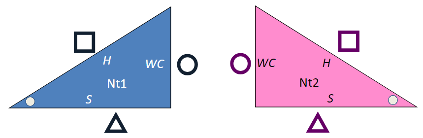

- If possible, print the diagram above and cut out the four triangles, leaving the white space containing the circle, square, and triangle symbols. Otherwise, do this mentally.
- Using one blue and one pink triangle, you can put the WC edges together to form a cis Watson-Crick/Watson-Crick basepair.
- With two copies of the blue triangle, you can put the Watson-Crick edges together in a different way, forming a trans Watson-Crick/Watson-Crick basepair.
- Using one blue and one pink triangle, you can form a cis H/H basepair, a cis S/S basepair, a trans H/WC basepair, and others.
- How many distinct basepairs can you form?
- Enumerating Basepairs using Triangle Bases
Exercise 5: Annotating RNA basepairs
View the 12 RNA basepairs at this link.
- Recognize whether the basepair is in cis or trans by looking at the glycosidic bonds, which connect the base to the ribose sugar.
- Looking at one basepair at a time, recognize and record the edges of each base that are interacting. Keep the edges in the same order as the bases!
- Write the 3-character annotation of the basepair after the base combination. When both bases are the same, make use of the nucleotide numbers as well.
- Write the bases in the opposite order and change the 3-character annotation to reflect the change in order.
- As a hint, the first basepair is UA tWH, which can also be written as AU tHW.
- Be patient, because the designation as cis or trans, or which edge is interacting, can be ambiguous. Over time it becomes more clear by comparing to the same base combination with a different geometry, or by comparing to a different base combination that is using the same edges.
Successive RNA basepairs
RNA basepairs are often made between successive bases in an RNA chain, for example in an RNA double helix or an RNA internal loop (which we will learn about in much more detail in the future). A first way to understand them is to list the covalently connected nucleotides in two columns, then draw arcs between basepaired nucleotides and write in the 3-character Leontis-Westhof annotation for the basepair, taking care to put the letters for the edges in the right order.
Exercise 6: Annotate successive RNA basepairs
View the collections of nucleotides at this link, one at a time.
- List out the covalently connected chains in two columns. Here is a guide for how to do that for the first collection of nucleotides. Note how the chains are listed in 5’ to 3’ order, which means increasing nucleotide numbers. For now, let’s put the lowest-numbered nucleotide in the lower left corner.

- Study the successive basepairs to determine which edges are being used in each pair, and write the three-character annotations on the two-column diagram.
Exercise 7: Form potential RNA basepairs from hydrogen bonding potential
- Print on paper two copies of each RNA nucleotide with hydrogen bonding potential shown. Use this link to get a PDF which shows both “top” and “bottom” views of each RNA base. Print both pages.
- Remember that for each base, the hydrogen bond acceptor groups are colored red, to reflect their overall negative charge. Hydrogen bond donor groups, made up of hydrogen atoms covalently bonded to electro-negative oxygen or nitrogen atoms, are colored blue, reflecting their overall positive charges. The 2’-OH groups are colored purple to indicate that they can serve either as hydrogen bond donors or acceptors and can interact with two groups simultaneously.
- Your goal is to find combinations of base edges that juxtapose hydrogen bond donors and acceptors so as to form at least two hydrogen bonds involving four atoms. Each red-colored functional group should partly overlap a blue-colored functional group while avoiding any red-with-red or blue-with-blue juxtapositions. There are 10 base combinations to explore. Pick one of the base combinations below, perhaps using the last digit of your phone number to choose from combination 0 to 9:
AC AG AU CG CU GU AA CC GG UU
- For the base combination you chose, find all possible orientations of the bases that will make at least two hydrogen bonds involving four atoms. Avoid structures where the glycosidic bonds (shown in red) fall on top of each other; the backbone is flexible, but not infinitely flexible. Sketch these on paper in such a way that it is clear what the relative orientations of the bases are, which hydrogen bonds are formed, and which face of the base is up.
- For the AA, CC, GG, and UU base combinations, you may need to print a second copy of each base. You can glue the top and bottom faces of each base together, if you like.
- Can you form a GG cWW basepair that makes two hydrogen bonds?
Exercise 8: Annotate RNA basepairs
- Annotate the 12 basepairs at this link by writing the base and number, 3-character Leontis-Westhof basepair code, and then the other base and number. Also write the interaction in the other order. Do your best with ambiguous cases. The most ambiguous case is number 9, and AC. Here are the AA, AC, AG, and AU basepairs in the same family, to give you a frame of reference. This is why the AC is also annotated as using the Sugar edge of the A, even though that is not obvious just from seeing the AC pair.
- Earlier, you pieced together two bases in different ways to form possible basepairs. Go through those again, discarding any that do not seem to really be basepairs, annotate them as cis or trans, and indicate what edges are being used.
Symbolic representation of base pairing
Leontis-Westhof basepair symbols
The 3-character annotation of RNA basepairs is nice for printed text, like in a paragraph in an article. Projecting RNA 3D structures onto a 2-dimensional diagram is also helpful, but it can be hard to orient text on a diagram to show clearly which base is using which edge in a basepair. In 2001, Leontis and Westhof introduced a simple set of geometric symbols to represent the base edges used and the glycosidic bond orientation:
- The Watson-Crick edge is represented by a circle
- The Hoogsteen edge is represented by a square
- The Sugar edge is represented by a triangle, with one point toward the base
- trans orientation is represented by “open” symbols (not filled in, as if they were transparent)
- cis orientation is represented by “closed” symbols, filled in
- A basepair is represented by a line from base to base, with the symbols on top of the line
- When both bases use the same edge, as in GU cWW, only one symbol is used
- For AU cWW, a single line with no symbols is used, following secondary structure convention.
- For GC cWW, a double line with no symbols is used, following secondary structure convention.
The following figure showing the Leontis-Westhof symbols appeared in a 2009 paper by Stombaugh, Zirbel, Westhof, and Leontis entitled “Frequency and isostericity of RNA base pairs,” which is available at this link.
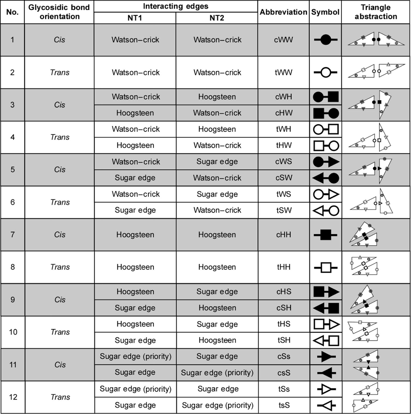
Figure 3. Annotations and symbols for non-Watson-Crick basepairs. From “Frequency and isostericity of RNA base pairs,” which is available at this link.
Exercise 9: Using Leontis-Westhof symbols
Add Leontis-Westhof symbols to the basepairs that you annotated in earlier exercises.
RNA Basepair Catalog
It is rewarding but difficult to annotate RNA basepairs by eye. One helpful resource is the RNA Basepair Catalog, which shows exemplar instances of each base combination in each of the 12 basepair families. Comparing to the Catalog is a good way to check annotations done by eye, and it’s a good way to know which base combinations have never been observed in RNA 3D structures.
RNA basepair annotations
The BGSU RNA Group’s website maintains annotations of basepairs and other interactions in all RNA-containing 3D structures. You can see the list of basepair annotations of a tRNA at this link. That link is for PDB file 1EHZ; by changing the URL, you can see annotations for any other RNA-containing file from PDB. Click on the three-letter code to see each basepair. Note that some three-letter codes are preceded by the letter “n”. This stands for “near” and indicates that it is plausible that the bases make the indicated pair, but the coordinates lie just outside the cutoffs for that pair. Perhaps a different structure determination experiment would show a true pair there.
RNA base stacking
Nearby bases that are not in the same plane are often in parallel planes, above and below each other, so that they overlap when viewed from above. This is called base stacking. As you look at the examples to follow, ask yourself to what extent the bases are truly in parallel planes.
Base faces
As with the Leontis-Westhof system for annotating basepairs, it is useful to annotate base stackings. A simple system for this purpose was introduced in the 2008 paper “FR3D: finding local and composite recurrent structural motifs in RNA 3D structures” by Sarver, Zirbel, Stombaugh, Mokdad, and Leontis, which is available at this link. The faces are named according to which direction they face in an RNA helix. The 3’ face is the one that faces toward the 3’ end of the chain (larger nucleotide numbers) while the 5’ face is the one that faces toward the 5’ end of the chain (smaller nucleotide numbers). The 3’ face is shown for each base in Figure 1 and in the left panel of Figure 2.
Base stacking annotation
When the 3’ face of one base stacks on the 5’ face of another base, we annotate this with the 3-character annotation s35, and similarly with other combinations of faces. The successive bases in an RNA helix make s35 stacking interactions. Some bases make cross-strand stacking interactions, which are not s35. In the exercise below, you will annotate base stackings as s35, s53, s33, or s55.
Exercise 9: Identify 3’ and 5’ faces of bases
View three successive basepairs from several RNA helices at this link.
- Starting with the lowest-numbered nucleotide, identify the 3’ face and 5’ face and check that the 3’ face stacks on the 5’ face of the next nucleotide.
- Look for cross-strand stacking, in which a base from one strand or chain stacks at least a little bit on a base from the other strand. What is the 3-character annotation for this stacking interaction?
- It is important to be able to identify the face of a base without using the nucleotide numbers of the neighboring nucleotides. Select a new instance, make sure that nucleotide numbering is off, and try to identify the 3’ and 5’ face of each base and determine which faces are stacking on which.
Exercise 10: Annotate base stacking
View several pairs of bases in different stacking orientations at this link.
- For each base, first find the Watson-Crick edge, then the 3’ face, then the 5’ face, then do the same for the next base and finally determine the stacking interaction.
- Annotate the stacking interactions as s35, s53, s33, or s55 stacking, being careful to list the bases and nucleotide numbers so that it is clear which base is using which edge.
Exercise 11: Annotate base stacking
Once again, view two collections of RNA nucleotides at this link.
- These are not standard RNA double helices, and there is no guarantee that all stacking between successive nucleotides is s35 stacking.
- Starting with the lowest-numbered nucleotide, identify the stacking interaction, if any, between successive nucleotides on each chain. You will probably benefit from finding the Watson-Crick edge of each base first, then the 3’ face, then the 5’ face, then do the same for the next base and finally determine the stacking interaction.
- Next, look for cross-strand or more complicated stacking interactions and annotate them.
Symbols for base stacking from François Major’s group
François Major of the University of Montreal led a focus group in the RNA Ontology Consortium focused on developing annotations for base stacking. One result was a symbolic system for annotated base stacks. Here are the symbols in terms of the base faces that we introduced earlier:
- s35 stacking is denoted >> and is called upward
- s53 stacking is denoted << and is called downward
- s33 stacking is denoted >< and is called inward
- s55 stacking is denoted <> and is called outward
These symbols are described in the 2007 paper by St-Onge, Thibault, Hamel, and Major entitled “Modeling RNA tertiary structure motifs by graph-grammars“ and available at this link. Here is the relevant text from the paper:
Two possible orientations of two stacked bases result in four base-stacking types: upward (>>), downward (<<), outward (<>) and inward (><). Two arrows pointing in the same direction (upward and downward) corresponds to the stacking type in the canonical A-RNA double-helix. Upward or downward is chosen depending on which base is referred first (i.e. A>>B means B is stacked upward of A, or A is stacked downward of B). The two other types are less frequent in RNAs, respectively inward (A><B; A or B is stacked inward of, respectively B or A) and outward (A<>B; A or B is stacked outward of, respectively B or A).
To further differentiate stacking from basepairing, the line connecting two stacked bases is often drawn as an elongated capital letter I, with the top and bottom of the I suggesting that the bases are in parallel planes.
Here is a useful way to remember: from the 3’ face, there is an arrow out from the base; from the 5’ face, the arrow points in, toward the base.
Suggestions for making 2-dimensional RNA interaction diagrams
It is very helpful to make 2-dimensional representations of RNA 3D structure. One cannot represent all of the detail of a 3D structure, but one can come close enough to gain real understanding of the 3D structure and make it easier to compare different small bits of RNA structures. Here are a few suggestions for how to lay out an RNA interaction diagram.Label the 5’ and 3’ ends of each strand and keep nucleotides from each strand together. This is especially important when sketching out a hypothetical or consensus motif that does not have nucleotide numbers on it. Put the 5’ end of one strand in the lower left corner.
- Put bases that make basepairs on the same horizontal level, as if they are in the same plane. The Sarcin-Ricin motif below has a base triple, with all three bases in the same plane,
- Put sequentially adjacent, stacked bases directly above/below one another, regardless of which faces are in contact. This has been done in the layout below, for example, with G75 and G76, which are next to each other in the nucleotide sequence and stacked.
- Use Leontis-Westhof symbols for basepairs.
- Use Major symbols for stacking. Note, however, that most diagrams do not have all stacking interactions annotated. The most important ones are stackings between non-sequential bases, especially stacking between strands, which should be indicated by elongated I bars. Extra space has been left above the base triple in the Sarcin-Ricin layout below to accommodate these bars.
Figure 4 below is a reasonable layout for the Sarcin-Ricin motif that we have been working with.
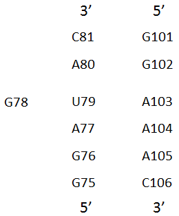
Figure 4. Layout for an interaction diagram for the Sarcin-Ricin loop.
Exercise 13: Annotating an RNA motif
Once again, view the two collections of RNA nucleotides at this link. Make symbolic interaction diagrams following the suggestions above. Use the layout suggested for the Sarcin-Ricin loop.
Base-phosphate interactions
In addition to the base-base hydrogen bonds that are present in RNA basepairs and that occur between the bases and the 2’-OH group on the sugar ring in some sugar edge basepairs, RNA bases often make hydrogen bonds with one or more of the oxygen atoms in the phosphate group of the same nucleotide or a different nucleotide. Many of these interactions are base specific, and so will play a part in establishing the relationship between RNA sequence and RNA 3D structure. These “base-phosphate interactions” were studied systematically in a 2009 paper by Zirbel, Sponer, Sponer, Stombaugh, and Leontis entitled “Classification and energetics of the base-phosphate interactions in RNA” and available at this link. The phosphate oxygens are highly electro-negative, so that any hydrogen atom on an RNA base could be the “donated” hydrogen in a hydrogen bond. The typical distance between a nitrogen atom in the base and the phosphate oxygen atom is around 3 Angstroms, while the typical distance when a carbon is the hydrogen donor is around 3.5 Angstroms. The phosphate oxygen is often out of the plane with the base, but the angle made by the nitrogen/carbon atom, hydrogen, and phosphate oxygen atom is usually greater than 130 degrees.
Base-phosphate interaction locations
Rather than use the base edge to describe the location of a base-phosphate interaction, the 2009 paper proposed a more detailed annotation of the location on each base where a base-phosphate interaction is made. Figure 5, which appears in the article, shows the possible locations and how they are numbered counterclockwise around the base. The numbering is done to facilitate noticing similar interactions being made by different bases. Note that the 0BPh interaction is in the same location for all bases. It is usually a self interaction, between the base and the phosphate of the same nucleotide. These are rarely annotated, but play an important role in the stability of many motifs. The 4BPh interaction is made only by G and involves two simultaneous hydrogen bonds, with one or two oxygens. Similarly, only C can make the 8BPh interaction. Note that base-phosphate interactions made by the Watson-Crick edge of G are particularly strong, these are 3BPh, 4BPh, and 5BPh.
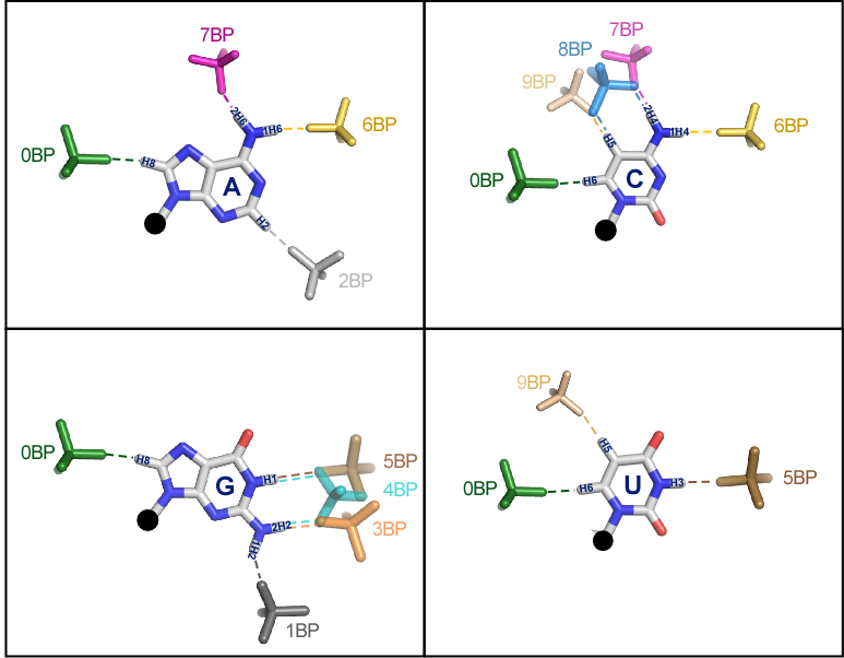
Figure 5. Possible locations of base-phosphate interactions for each of the RNA bases. From the paper “Classification and energetics of the base-phosphate interactions in RNA” which is available at this link.
Base-phosphate interaction and the assignment of atoms to nucleotides
The four oxygens attached to the phosphorus of a nucleotide are called O5’, OP1, OP2, and O3’. In RNA 3D structures, if the phosphorus is part of nucleotide N, then O5’, OP1, and OP2 are part of nucleotide N as well, but O3’ is part of nucleotide N-1. In visualizations, O3’ may or may not appear together with nucleotide N. In the 3D coordinate viewers available in this course, you can hover over each atom to see the atom name.
Base-phosphate interaction character annotation
As with basepairs, one specifies a base-phosphate interaction by listing the two bases involved. Because of the asymmetry of the interaction, it is typical to always list the nucleotide (base) which acts as a hydrogen bond donor first, then the nucleotide whose phosphate oxygen is the hydrogen bond acceptor. Thus, for example, we may have G14 5BPh U27 when G14 uses its H1 atom as a hydrogen bond donor to the phosphate group of nucleotide U27.
Base-phosphate interaction symbolic annotation
Starting with the 2009 paper on base-phosphate interactions, the main way to annotate these interactions is with with a “barbell” consisting of an open circle with P inside, for the nucleotide whose phosphate is used, and a filled circle with the number of the base-phosphate interaction (0 to 9) in white, as below.
Figure 6. Symbol for annotating a 5BPh interaction.
Exercise 14: Annotate base-phosphate interactions
View the 18 pairs of bases at this link.
- Identify the base-phosphate interaction(s) being made and annotate them using characters like “5BPh”. Note that some interactions are made with the O3’ atom, which is not shown with the nucleotide whose phosphate oxygen is the hydrogen bond acceptor. You may need to view the neighborhood to see clearly where the hydrogen bond is made. Bonus points for identifying the oxygen atom which is the hydrogen bond acceptor.
Exercise 15: Annotate base-phosphate interactions in a helix
Return to the 6-nucleotide RNA helices at this link.
- Each base makes a self base-phosphate interaction. Identify the location of this interaction (0 to 9) and, if you can, the phosphate oxygen that is the hydrogen bond acceptor.
- Measure the distances between the hydrogen on the base and the phosphate oxygens by double clicking the hydrogen and then double clicking an oxygen. How consistent are these distances from one nucleotide to the next?
- Measure the angles between the heavy atom on the base, the base hydrogen, and the phosphate oxygens. Hydrogen bonds prefer a bond angle around 180 degrees.
- Comment on the contribution of base-phosphate interactions to the stability of the double helix.
- Comment on the base specificity of the base-phosphate interaction in a double helix.
Exercise 16: Annotate base-phosphate interactions in a motif
Return to the two collections of RNA nucleotides at this link.
- Find all self base-phosphate interactions in the two instances. A good strategy might be to focus on each phosphate group in turn and see if a base is interacting with it.
- Find all inter-nucleotide base-phosphate interactions in the two instances.
- Add the base-phosphate interactions to the symbolic annotations that you made in Exercise 9.
Exercise 17: Extended investigation of basepairs
Read two articles by Leontis and Westhof about RNA basepairs. They are:
- Geometric nomenclature and classification of RNA base pairs, 2001, available at this link
- The non‐Watson–Crick base pairs and their associated isostericity matrices, 2002, available at this link
Keep notes as you read. Here are some things to focus on, in addition to whatever else you want to write:
- In the 2001 paper, make note of topics that we did not cover previously.
- In the 2001 paper, how do you determine which way the triangle points in cSS and tSS interactions? Write this out in your own words.
- The 2001 paper is a sales pitch, trying to sell a new way to annotate basepairs. What do you think are the most effective arguments for this system of annotation? Can you anticipate any drawbacks to this system? (I recognize that until you look at a large, large number of basepairs, you can’t really evaluate the limitations of the method, but at least you may have some concerns.)
- For the 2002 paper, it’s not really worth printing out the 12 tables of basepairs. Instead, use the RNA basepair catalog at this link. The basepair catalog has basepair “exemplars” and observed counts from all high-resolution structures from 2011. You will need to enable Java applets for the Jmol applets on that page.
- After the tables of basepairs, the 2002 paper discusses each family of basepairs and which base combinations within them are isosteric. Write out a one- or two-sentence definition of the word “isostericity” in this context. Then, read the paragraphs about the cWW basepair on pages 3526 and 3527. Also, read about one additional family and become an expert on it by completing the next two points.
- For your chosen basepair family, count the number of hydrogen bonds and estimate the strength of the hydrogen bonds made by each base combination (AA, AC, AG, etc.). Compare these to the counts of the number of occurrences. You will find occurrence counts from 2011 in the RNA basepair catalog at this link. Do the more common base combinations have more hydrogen bonds and/or stronger hydrogen bonds?
- You may remember that for some of the basepairs that we annotated at this link, it was not very clear whether they were cis or trans. For your assigned basepair family, look at all of the base combinations. Do all of the base combinations belong in the same family? Does the annotation as cis or trans make sense, when you look at all base combinations together?
Anti versus syn conformation of the glycosidic bond
The glycosidic bond, which connects the RNA base to the ribose sugar ring, allows for 360 degrees of rotation around the bond, so that the geometry of the base and the sugar could be quite variable. However, it turns out that most RNA bases have roughly the same orientation between the base and sugar, as characterized by the conformation of the ribose sugar in the standard RNA helix. This is called the anti conformation. Around 4% of all nucleotides have a completely different orientation, called syn, in which the phosphate group of the nucleotide is closer to the sugar edge. The purpose of the following exercises is simply to help you see the difference between clear examples of the two glycosidic bond conformations.
Exercise 18: Anti and syn in RNA helices
View some standard RNA helices at this link.
- Check that all ribose sugars have the same orientation with respect to the bases for all six nucleotides in the first few instances. Note the self base-phosphate interactions made by each base. What features of the ribose or backbone can you use to recognize this glycosidic bond conformation?
Exercise 19: Annotate anti and syn conformation
View 11 nucleotides with different glycosidic bond conformations at this link.
- Most of the nucleotides have a clear glycosidic bond conformation. Label them as being syn or anti.
- Some of the nucleotides have an ambiguous glycosidic bond conformation. Look at the C4’-C5’ bond to see if that provides any clarity on how to annotate them, but don’t worry about it getting it “right” because there really is no right answer. (Turn on atom names by right clicking and choosing Style, Labels, With Atom Name.) If you really want to see where the dividing lines are between annotations that people make, look at the examples of bases with the glycosidic bond at different dihedral angles, with 5-degree steps or with 2-degree steps.
Exercise 20: Annotate anti and syn in an RNA motif
Return to the two collections of RNA nucleotides at this link.
- In the first instance, all ribose sugars appear to be consistently on the same side of each base, but recall that some consecutive stacking interactions are not the typical s35 stacking, so at least one of the glycosidic bonds is in the syn conformation. Which one or ones? How can you tell?
- In the second instance (Sarcin-Ricin motif), check through all nucleotides to see which ones, if any, are in the syn conformation.
- The Sarcin-Ricin motif is often called the “S-turn”. Can you find the part of the backbone that is called the “S-turn”?
Exercise 21: Annotate anti and syn in an RNA motif
View 7 instances of a new internal loop motif at this link.
- Draw an interaction diagram for the first instance, putting the lowest-numbered nucleotide in the lower left as usual, labeling the 5’ and 3’ ends of each strand, etc. Use Leontis-Westhof symbols for the basepairs. If you have time, annotate any unusual stacking and/or base-phosphate interactions.
- Neocles Leontis (personal communication) says that one base in one instance is modeled in syn, which is wrong. Find that base and give arguments to support the claim that it is modeled in syn and that this is wrong. It may help to know that many of these instances are from ribosomal structures, but as it happens, they are not all from homologous locations.
Experimentally determined RNA 3D structures
This section gives an overview of the RNA-containing 3D structures available for download.
Where can one get RNA 3D structures?
As a condition of publication, atomic-resolution 3D structures of biological molecules are deposited with the worldwide Protein Data Bank (wwPDB), which has four members: PDB in the US, PDBe in Europe, PDBj in Japan, and BMRB for NMR structures. One can visit any of these sites to explore what 3D structures are available. The Nucleic Acid Knowledgebase (NAKB) is a close partner of the BGSU RNA group, with additional search and viewing features. PDB101 is an educational site about 3D structure data, and the section Introduction to PDB Data is particularly useful for the details of 3D structure.
Tour of RNA 3D structures using Representative Sets
In order to give an overview of what structures are available, please follow along with this tour of the BGSU RNA Group’s page for Representative Sets of RNA 3D Structures.
- Start at this link, entitled Representative Sets of RNA 3D Structures. You can easily find this page by searching for “RNA representative set” or “nrlist” (for non-redundant list). This page is updated every week with new RNA 3D structures downloaded from PDB. The table shows the 5-fold growth in the number of RNA-containing 3D structures from 2011 to 2018. It indicates that there are now over 10,000 RNA-containing 3D structures, which are organized into around 9,000 IFEs, or Integrated Functional Elements. These are either one RNA chain or multiple RNA chains strongly connected by Watson-Crick basepairing. We’ll see examples later in the tour.
- Click on the current release. This shows a large table of RNA 3D structures. To simplify things, click on the 1.5A tab above the table. This restricts the view to RNA 3D structures solved at 1.5 Angstrom resolution or better. The length of a carbon-carbon bond is about 1 Angstrom, so these structures are able to resolve essentially all of the atoms in a 3D structure with little to no guesswork.
- Each row of the table shows a distinct RNA molecule. The largest entry is at the top. As of October 2018, the largest entry solved at this resolution has 67 nucleotides. Click on one of the 4-character PDB identifiers to see a popup window that tells more about the molecule.
- The rightmost column illustrates an important feature of the PDB: the same molecule may have been solved experimentally more than once. What is the highest number of structures of the same molecule on this page? It’s more than 18. The PDB IDs in the rightmost column are listed in decreasing order of overall structure quality, as measured by a combination of factors including resolution, steric clashes, and how well the atoms fit the experimental data. Click a PDB ID and look for the CQS score. Lower is better.
- The Representative column lists the structure with the lowest Composite Quality Score, which is taken to be the representative structure for that molecule. This is a good structure to look at first. The collection of all representative structures gives a representative set, as in the title of the page.
- Clicking on the columns sorts the rows of the table. What is the best resolution available here? (The lowest number in the resolution column.)
- The filter box restricts what rows of the table are shown. Are there any full tRNA structures in the 1.5 Angstrom set?
- Click the 2.0A tab to relax the resolution cutoff a bit, and look again for tRNA structures. The 1.2A structure is still there, but it is joined by other structures with proper lengths for a tRNA. What organisms do these structures come from?
- Click the first tRNA structure listed in the 2.0A representative. In October 2018, that is 3R5G, model 1, chain B. (There is also a chain A in the same structure. Can you tell why chain B was chosen as the representative, from the Structure Quality data in the popup?)
- At the bottom of the popup are links to view the structure at PDB, NDB, and the BGSU RNA site. Let’s start at the PDB entry. The direct link is https://www.rcsb.org/structure/3RG5 When was this structure released?
- In the left-hand column, next to 3D View, you can click to view the structure, the electron density, and the ligand interaction. Click to view the structure first. Click to make it Fullscreen. Try the different Style choices in the right-hand column. Licorice and Line are the views we have seen with RNA basepairs, showing the atomic bonds, but the other views also give insight. The Line view shows double bonds as well.
- At the top of the right-hand column, click the Electron Density Maps to view the experimental electron density data.
- Return to the 2.0A Representative set, click the first tRNA structure, and now select to view the structure on the BGSU RNA site. The direct link is http://rna.bgsu.edu/rna3dhub/pdb/3RG5
- Click the Interactions tab, then Base-pair. This lists the basepairing interactions in the structure, according to the unit ID of each nucleotide. The format of the first unit ID, 3RG5|1|A|G|1, goes like this:
- 3RG5 is the PDB identifier
- 1 is the model number, usually 1 for x-ray structures like this one
- A is the chain
- G is the base
- 1 is a text string that usually looks like a number and is usually sequential
- The BGSU RNA site uses unit IDs wherever possible as a unique way to refer to a specific nucleotide or amino acid in a particular structure. You can read about them at https://www.bgsu.edu/research/rna/help/rna-3d-hub-help/unit-ids.html or by click on a unit ID and choosing Nomenclature.
- Looking a little farther down the list, there are three nucleotides that are number 5! The second one has an “insertion code” A at the end, the third one has insertion code B.
- After all of the base-pair interactions from Chain A, Chain B is listed. Note that there must be a version of Chain B that was produced by symmetry operation 1_556. This has to do with crystal symmetries and is beyond the scope of this course, but suffice it to say that due to how x-ray crystallography works, sometimes you need to apply symmetry operators to get the whole view of the molecule.
- Click on the 2D Diagram tab on the page for 3RG5. This shows the nucleotides of chains A and B arranged clockwise around a circle, starting at the top of the circle. Hover over the black outer circle to identify the nucleotides. Hover over a black arc to see Watson-Crick basepairs and which bases make them. Nested arcs indicate Watson-Crick double helices. Click and drag a rectangle to view the 3D coordinates of a whole chain or just part of a chain. Click the All button on the left side to view RNA basepairs from all 12 families.
- Return to the Representative Set page and click on the 3.0A tab. There are much larger structures solved to this resolution, including many full ribosomes. Filter by “sapiens” to find the RNA molecules from Homo sapiens that are solved to 3.0A resolution or better. Is there a complete ribosome? Yes, from PDB ID 6EK0 (the last character is the number 0). Filter by 6EK0 to see what chains are in that 3D structure. Note that the large ribosomal subunit is made up of two chains. What are the chain identifiers? They are not single letters; chain identifiers can be up to 4 characters long.
- Have a look at the 2D Diagram for the Homo sapiens ribosome. The longest chain (L5) makes a significant number of Watson-Crick pairs with a shorter chain, L8, called the 5.8S rRNA. For that reason, they are kept together as an Integrated Functional Element. What chain is the Small Subunit (SSU)?
- Click to show all RNA basepairs, and note how many basepairs cross over the Watson-Crick double helices. This is a sign that the network of interactions that holds together a large RNA like the ribosome is very complicated, and that distant parts of the RNA sequence must be statistically dependent on one another, to maintain the correct basepairs.
- Return to the Representative Set page at resolution threshold 3.0A. Scroll down to see rows for ribosomes from E. coli and T. thermophilus. Note the long list of structures in the right-hand column, which are all structures of essentially the same molecule, but typically under different experimental conditions, with much older structures typically lower on the list. Recognizing this redundancy and recommending a single structure to study is a key benefit of the Representative Sets.
- Finally, return to the Representative Set page and click on the All tab. This shows all RNA-containing 3D structures, including those solved by solution NMR. Filter by NMR to see that there are around 572 NMR 3D structures.
RNA 3D Motif Atlas
Of particular interest in RNA are the portions between the helices and at the ends of the helices. The tutorial at this link will orient you to RNA hairpin, internal, and multi-helix junction loops. The RNA 3D Motif Atlas collects together all internal loop and hairpin loop instances from across a 4.0A representative set of RNA 3D structures and collects together instances into motif groups, with the goal that within each motif group, all instances are instances of the same motif. Due to the natural variability of RNA molecules, there is some variability in the geometry within each group, but overall, the clustering is successful. Ideally, the Motif Atlas is updated every four weeks. It is helpful to be aware of at least some of these groups, so please follow the links below.
- The current internal loop families are at this link. The groups are listed in decreasing order of number of instances, and the largest groups are not particularly interesting, so scroll down a bit, looking at the basepair diagrams on the left side to get an idea what basepairs the loop is made up of.
- The “triple sheared pair” motif is a nice one, see http://rna.bgsu.edu/rna3dhub/motif/view/IL_56467.9 There are 35 instances from many different structures, and non-homologous places in those structures. The table on the right lists the instances, with corresponding nucleotides aligned in each column. Scrolling to the right, you will see that most instances have conserved tHS and tSH basepairs, but that some do not have all three basepairs annotated.
- You can view individual instances by directly selecting them, clicking Next or Previous, or by using the heat map in the lower right.
- The heat map in the lower right shows all-against-all geometric discrepancy between the motif instances. Warm colors mean the instances are geometrically similar. The instances are ordered so that similar instances are near one another in the list, putting the warm colors near the diagonal. Hover over the heat map to see which instances are being compared in each cell of the heat map. Click the heat map to see the two instances superimposed. Reorder the listing in the table by clicking the #S column header to list the instances in the same order as they are listed in the heat map.
Sequence variability in structured RNA molecules
DNA is not always copied perfectly when organisms reproduce. The two main types of errors that we consider in this course are mutations and insertion/deletions (indels). At the moment, the focus is on mutations, a change from one nucleotide in a DNA position to a different one. Among other things, this can result in a base change in a structured RNA molecule. Roughly speaking, there are three possibilities: the mutation can disrupt the structure of the RNA molecule to such a point that the offspring cannot survive or cannot reproduce, and so we do not see these mutations in living organisms. Occasionally, the mutation may confer a survival advantage to the organism, the offspring of the organism may outcompete others in its species, and so this mutation may become fixed in a population. The third possibility is that the mutation has no significant effect on the performance of the structured RNA, in which case the mutation may come to exist in the population at some level between 0% and 100%. These are called “neutral” mutations, although some might be slightly advantageous and others slightly disadvantageous. These are the most commonly-observed types of mutations.
Nucleotide to nucleotide alignments of RNA 3D structures
The first step in understanding typical sequence variability in structured RNA molecules is to compare 3D structures of homologous molecules, ones that share a common ancestry. See our new tools in 2024 which are described at https://www.bgsu.edu/research/rna/web-applications/r3d-align.html The basic idea of the alignments is to identify nucleotides in each structure which correspond geometrically in the sense that their local 3D neighborhoods have the same local 3D neighborhood in the other structure.
Exercise 22 - needs to be rewritten
Start at the R3D Align Gallery of Featured Alignments at this link.
- View the alignment between ribosomal 5S RNA from E. coli and T. thermophilus by clicking on the image in the corresponding row and column. These are both bacteria, but have been reproducing separately for over 1 billion years.
- By clicking the button labeled “Hide unaligned nucleotides” you can find nucleotides that are not part of the alignment. Look for A15 in each structure and note how it is modeled differently. This helps to explain why it is not part of the alignment.
- Spend some time looking at the aligned nucleotides. Look for cases in which the nucleotides are not the same between the two structures (although this is difficult because one structure is blue and the other is orange).
- Note that R3D Align produces a nucleotide to nucleotide alignment, but the visualization uses a single rigid translation and rotation to superimpose the structures. Aligned nucleotides far from the center, in particular, do not superimpose all that well, but they do have the same orientation.
- Click on the tab labeled “Basepairs” to see the nucleotide to nucleotide alignment and, for each nucleotide making a basepair, the corresponding basepair in the other structure, if any.
- Scroll down through the list of aligned bases and basepairs. Note that C12 and A15 are not aligned, even though they have the same base and would be aligned by a sequence-based alignment program.
- Note the degree of conservation of basepair family between the two structures, and also instances of non-conservation. For example, G69-G107 makes a tSH basepair in E. coli (2QBG) but it is aligned to G69-U108 in T. thermophilus, which makes a cWW basepair. Where in the 3D structure does this pair occur?
We will look more at alignments of 3D structures later. The point now is that we can directly examine the structures and see (with more work) that in the vast majority of cases, basepairing family is conserved between 3D structures of homologous organisms.
RNA Basepair isostericity
A well-known example of neutral mutations in RNA basepairs is the covariation of bases in cis Watson-Crick / Watson-Crick basepairs in RNA helices. Looking at a multiple sequence alignment of RNA homologous sequences (same molecule, different organisms, but where the molecule first arose from a common ancestor), one will often observe changes between the “canonical” base combinations AU, UA, CG, and GC in two columns whose nucleotides make a cWW basepair. It is important to note that, because the two nucleotides making a cWW basepair will tend to be at least 6 positions away from one another in the RNA sequence (enough sequence length to form a hairpin loop), and are often much further away in sequence, it cannot be assumed that both mutations happen at the same time, but rather that one happens and is tolerated, and that in a later generation, the compensatory mutation occurs. Thus, cWW covariation has implicit in it the possibility of non-matched basepairs occurring in RNA helices (these are often called “mismatches,” but that is probably a good word to avoid as it does not really explain what is happening; a “mismatch” could form an important non-canonical basepair), at least for a number of generations.
The purpose of this section is to explore the basis for Watson-Crick covariation and to extend the observations we make there to other RNA basepairs, in order to make predictions about likely and unlikely sequence variability in structured RNA molecules.
Choosing basepair exemplars from each basepairing family
One good place to start examining the geometric similarities between RNA basepairs is to have “exemplar” instances of each base combination in each basepairing family. To this end, all instances of each base combination for each basepairing family were extracted from a non-redundant set of RNA-containing 3D structure files determined by x-ray crystallography with resolution 4.0 Angstroms or better. (As of 2013-11-25, structures with extension .pdb1 were excluded from this analysis.) Geometric discrepancies were calculated between each pair of basepairs, as described in the 2008 article “FR3D: finding local and composite recurrent structural motifs in RNA 3D structures” by Michael Sarver, Craig L. Zirbel, Jesse Stombaugh, Ali Mokdad, Neocles B. Leontis, which is available at this link. Basepairs whose bases are “coplanar” as defined in the 2011 article “Comprehensive survey and geometric classification of base triples in RNA structures” by Amal S. Abu Almakarem, Anton I. Petrov, Jesse Stombaugh, Craig L. Zirbel and Neocles B. Leontis, which is available at this link were separated from those which are “non-coplanar”. If there is at least one coplanar basepair, the coplanar instance which minimizes the product of the reported resolution of the structure, the sum of discrepancies to all other instances, and the numerical rank of the candidate when listed by the sum of discrepancies to all other instances, is chosen as the exemplar. If there is no coplanar instance, the same ranking is applied to the coplanar instances, or else a curated instance is used.
RNA Basepair Catalog
The exemplar basepairs are displayed in the RNA Basepair Catalog hosted at the Nucleic Acid Knowledgebase; it is available at this link. For each basepairing family, instances of each known base combination making the basepair are shown. This is a very useful reference to be able to see the best known instances of each base combination in each of the 12 basepairing families.
Displaying basepair exemplars from each geometric basepairing family
The basepair exemplars from each geometric basepairing family are shown in a single PDF, available at this link. The families are listed in the same order as in the 2002 paper by Leontis, Stombaugh, and Westhof. Thus, cWW starts on page 1, tWW on page 4, cWH on page 7, tWH on page 10, cWS on page 13, tWS on page 16, cHH on page 19, tHH on page 22, cHS on page 25, tHS on page 28, cSS on page 31, and tSS on page 34. Above each basepair is a title which indicates the base combination, the PDB ID of the 3D structure it is taken from, the nucleotide numbers within that structure (but not the chain), the distance in Angstroms between the C1’ atoms of the two nucleotides, and the number of instances of this base combination in the non-redundant set from which the exemplars were drawn.
Some notes about the basepairs.
- The cWW basepairs on page 1 have three base combinations on the diagonal, AA, CC, and UU. Please note that these are not symmetric, and so uppercase and lowercase W’s have been used to indicated which base is “first” and which is “second” in this pair.
- The first base in each base combination is put in the same orientation across each row of instances.
- If you want to be able to zoom in on a base combination or rotate it, please visit the RNA Basepair Catalog at this link.
- RNA molecules are in constant motion in the cell, as they are surrounded by water and other molecules which are moving and bumping into each other. The hydrogen bonds that maintain RNA basepairs are not as strong or rigid as covalent bonds, and so it can be expected that the relative orientations of RNA bases will change from moment to moment. It should be reasonable to think of the basepair exemplars as giving a pretty good idea of the nominal relative orientation of the two bases, something like a ground state or energy minimum.
Position of glycosidic bonds in RNA basepairs in the same geometric family
On page 1, take a moment to compare the glycosidic bonds on the AU, CG, GC, and UA cWW basepairs. These appear diagonally from upper right to lower left. The glycosidic bond of the first nucleotide is always vertical, so focus on the relative location and orientation of the second one. You can see that the orientation (angle) is roughly the same in each case. Also, note from the title above each instance that the C1’-C1’ distances are nearly the same, 10.6 Angstroms for GC and CG, and 10.4 Angstroms for UA and AU. To really be able to focus on the relative orientations of the glycosidic bonds, go to a later page which shows just the glycosidic bonds for the base combinations in the cWW family. The glycosidic bonds of the first base are all superimposed in the lower left, so that you can compare how different the relative positions of the glycosidic bonds of the second bases are. Note how close in the plane the second glycosidic bond in the AU, UA, GC, and CG base combinations are. Note that their orientations (angle with respect to horizontal) are identical. As far as we know, this is one of the reasons that one frequently sees substitutions between AU, UA, GC and CG in RNA helices: substituting one base combination for another need not disturb the RNA backbone at all.
Now find the glycosidic bonds of the GU and UG cWW basepairs. They are at a considerable distance from the AU, UA, CG, and GC bonds, although they have the same orientation. Note, in particular, that the glycosidic bonds from GU and UG are really far apart from each other. This explains how it is that occasionally one sees a GU or a UG substituting for a canonical cWW basepair in an RNA helix. But there are other locations where, for some reason, a UG or a GU cWW is preferred, and there one does not often see the base combination in the other order.
IsoDiscrepancy Index to measure the degree of isostericity between two basepairs
In the 2009 paper, “Frequency and isostericity of RNA base pairs” by Jesse Stombaugh, Craig L. Zirbel, Eric Westhof, and Neocles B. Leontis which is available at this link, a quantitative measure of basepair isostericity was defined and called “IsoDiscrepancy Index” or IDI. The idea is to make a score that increases the more dissimilar the glycosidic bonds are. The images below are reproduced from the 2009 paper and show the three contributions.
These three measurements are combined as explained in the 2009 paper to calculate the IDI between different instances of RNA basepairs. The exact details need not concern us here.
IsoDiscrepancy values within each geometric basepairing family
The same PDF that shows instances of each basepair also shows calculated values of the IsoDiscrepancy Index between exemplars, in a colorful matrix. The cells in the matrix are colored according to the IDI value, using the scale at the right of the matrix. The numerical value also appears in each cell. Base combinations are ordered the same in the rows as in the columns, and the ordering is chosen to put similar base combinations near each other in the list, so as to put more of the small IDI values near the diagonal.
Look at the IDI matrix for the cWW family and confirm that the mutually isosteric subgroups match your expectations from the superpositions of glycosidic bonds and the basepair exemplars themselves.
Exercise 23
- View three instances of a kink-turn motif at this link. The goal is to annotate each of them completely.
- Start by identifying the cWW basepairs that flank each kink turn, and note that the helices that they begin (not shown) will exit the kink turn at quite different angles. This is why this motif is called a kink turn.
- You might want to use a pencil and have an eraser ready.
- Turn on nucleotide numbers so that you can draw a schematic diagram of the nucleotides and the interactions they make. Put the nucleotide number listed next to the checkbox for each structure in the lower left; the numbers are 1312, 277, and 121. Then list out the rest of the nucleotides.
- Keep an eye on the basepairs when you list the nucleotides in the second strand, so you can put them next to their basepairing partners.
- In the second instance, I would recommend listing the nucleotides in the second strand out of order, using arrows to show how the backbone is connected. This will make the basepairs horizontal.
- There are four bulged nucleotides in the three instances; list these to the side so that it’s clear that they are bulged out of the motif.
- Do your best to identify each of the basepairs present in the two motifs. Some of them are not as planar as the ones we have classified in the past, so put them in the closest category. In particular, 1313-1341, 277-282, 246-278, 197-200, 121-123 are tricky sugar edge basepairs, but very important because they hold the “kink” together. Remember that in sugar edge basepairs, the triangle points toward the base that interacts with the O2’ on the ribose of the other base.
- Check each nucleotide to see if it is in syn or anti. If syn, circle the nucleotide letter. If ambiguous, underline the nucleotide letter.
- Stacking is important in a motif with a tight bend like a kink turn, but annotating all of the stacking interactions is a challenge. Can you do it? Some stackings have only a small overlap; you can annotate them with a dotted line.
- The first instance has a nice base-phosphate interaction. Find it and annotate it.
- If your diagram is a mess, now would be a good time to redraw it.
- What do these three kink turns have in common?
- Start reading the 2009 paper, “Frequency and isostericity of RNA base pairs” by Jesse Stombaugh, Craig L. Zirbel, Eric Westhof, and Neocles B. Leontis which is available at this link. In class we will continue discussing the definition and use of the Isostericity Discrepancy Index (IDI) and how to use isostericity to understand sequence variability in structured RNA molecules.
RNA secondary structure
RNA molecules are made by transcription from DNA, which joins together the four RNA nucleotides A, C, G, and U in the order given by the DNA strand that is being transcribed. Transcription is said to go in 5’ to 3’ order; these numbers refer to the O5’ and O3’ oxygen atoms on the RNA backbone and this gives a standard sense of direction along the RNA chain. In RNA 3D structures, the nucleotides are always numbered in increasing order, following 5’ to 3’ order. The sequence of nucleotides is called the primary structure. For most RNA molecules, the primary structure is all that is known from direct experimental evidence, usually genome sequencing.
Even while the rest of the RNA molecule is being transcribed, the nucleotides that are already transcribed are moved about randomly by the molecular motion of water in the cell and occasionally two strands will come together and form a sequence of cWW basepairs, which will then form themselves into an RNA helix. We have seen portions of RNA helices in earlier exercises and you can see them again at this link. By far the most common base combination to form cWW basepairs is GC (7478 instances), followed by AU (2641 instances), with GU a distant third place (796 instances). GC and AU base combinations are often called canonical while GU is called wobble. In structured RNA molecules, RNA helices typically consist of between 2 to 10 stacked cWW basepairs. The list of GC, AU, and GU Watson-Crick basepairs in RNA helices is called the secondary structure of an RNA. (Pro tip: in some structures, some Watson-Crick basepairs “cross” others, forming pseudoknots. That is a subject for a later discussion.)
Exercise 24
Re-visit the short RNA helices at this link.
- Write out the nucleotides in the first instance and make a basepairing diagram like we have done for other collections of RNA nucleotides, starting with U86 in the lower left.
- Note that U86, the lowest-numbered nucleotide in the first strand, pairs with A108, the highest-numbered nucleotide in the second strand. While the backbones twist to make a helix, they run in opposite directions, so we say that the strands here are anti-parallel.
- Note the large jump in nucleotide numbers from C88 to G106. Many nucleotides have been omitted from this fragment of a 3D structure. In many ways, RNA molecules are modular, and it makes sense to look at small portions of them at a time.
- It is helpful to list out the bases in this RNA fragment as UGC*GCA. The bases are listed in 5’ to 3’ order, with the * representing a break in the chain. Write down this sequence of letters and draw circular arcs between the bases that make cWW basepairs.
- Note that the arcs you drew in the previous step do not cross each other. They are said to be nested.
Interactive RNA secondary structure
Each RNA-containing 3D structure has a web page on the BGSU RNA Group website. Each such page includes a viewer for the secondary structure. A key feature of the viewer is that after selecting portions of the secondary structure, a window opens to display the corresponding nucleotides in 3D.
One of the most common and most often studied structured RNAs is tRNA, or transfer RNA. tRNAs help in the process of protein synthesis, called translation, by bringing the correct amino acid to the right place on the ribosome at the right time. Many tRNA 3D structures have been solved, but they differ from one another in small ways.
Exercise 25: Analysis of a tRNA structure
Open the 2D diagram for the tRNA molecule in PDB file 2CV1 at this link.
- The nucleotides of the RNA are arranged clockwise around a circle. Hovering over the circle will display the base and nucleotide number.
- By default, the first view after loading shows the cWW basepairs as black arcs. Hovering over an arc will display the two nucleotides that make the basepair. Note that there are four collections of successive basepairs, and so four RNA helices. Note how the arcs are nested one inside the other.
- Clicking the arc for a basepair will cause the nucleotides to be displayed in the window to the right. From there, you can display the nearby nucleotides by clicking Show Neighborhood. Note that the basepair is listed in text format below the 3D window.
- Click and drag on the circular diagram to make a rectangle that contains the nucleotides that make up the longest helix. You will get some additional nucleotides as well. Confirm that all of the basepairs are cWW. Check the other helices as well. What is the most common base combination? How many GU basepairs are present?
- Three of the helices have a hairpin loop at the end. This is a connected strand of nucleotides that bends back on itself. Select each of these helices and the hairpin loop at the end, and see what kind of structure the hairpins have, if any.
- There is a cWW basepair between C556 in what is called the T-loop and G519 in what is called the D-loop. The arc for this interaction crosses many other cWW arcs, so this interaction is unlike the other cWW basepairs. This is why the arc is drawn as a dashed line, not solid. Interactions like this are generally not considered to be part of the secondary structure; they are called long-range interactions. Visualize the T-loop in the 3D viewing window and click Show Neighborhood to confirm the cWW basepair.
- There is another long-range interaction between U555 and G518. What kind of basepair is this?
- The four helices are connected to one another by a 4-way junction. It is not easy to visualize the 4-way junction in this viewer, but it consists of the nucleotides A507 to G510, G525 to G526, A544 to G549, and C565 to U566. We will work on junctions later in the course.
- There is another cWW basepair between C548 and U520. Keep in mind that hairpins can interact with junctions. Unfortunately, not much is known about these interactions in general.
- Clicking on the All button to the left of the circular diagram will add arcs for all other RNA basepairs in the structure. Note the tWW basepair between C548 and G515. Thus, C548 makes two basepairs at once, and so is part of a base triple. Again, hairpins can interact with the nucleotides in a junction.
- Select and view nucleotides C561 to C572. These belong to two different RNA helices, but notice how their backbone forms an unbroken helix of its own nevertheless. Click Show Neighborhood and see if you can tell how the two helices come together. This is called co-axial stacking of helices. Where else does something like this happen in the tRNA?
Exercise 26: The T-loop
Transfer RNA has a hairpin loop known as the T-loop, probably because in tRNA it contains a modified nucleotide (thymidine), but it also fits that the T-loop occurs in tRNA. The same type of hairpin also occurs in ribosomal RNA, some riboswitches, and other structured RNAs.
- Starting with the circular diagram for 2CV1 at this link, visualize the T-loop in 3D from G553 to C561 and answer the next few questions.
- In the T-loop in 2CV1, what basepair is made between U554 and A558?
- In the T-loop in 2CV1, U555 is held in place by a base-phosphate interaction. What type of BPh is it?
- You can see many T-loops aligned to one another at this link. This is called the T-loop motif group, and it has HL_72498 as its identifier. Most of the T-loop instances here come from tRNAs, but some come from ribosomal RNAs. The next several questions concern base conservation across T-loop instances.
- The basepair between U554 and A558 corresponds to the nucleotides in columns 2 and 6 in the T-loop motif group. What base combinations do you see in these two columns? To the right of the columns of aligned nucleotides are annotations of the basepairs in each instance. How do the basepair annotations relate to the base combinations?
- Nucleotide U555 in 2CV1 corresponds to nucleotide 3 in motif group HL_72498. This nucleotide is not perfectly conserved across the different instances. Is the base-phosphate interaction conserved?
- You can put the instances of the T-loop into a very useful order by clicking the #S header of the second column once. This puts the instances into similarity order, which means that geometrically similar instances are placed near each other in the list. This is the order that is used to make the heat map in the lower right of the page. In the heat map, you may notice a large cluster of instances whose mutual geometric discrepancy is relatively low, shown as dark orange. Below this is a smaller cluster of instances.
- Compare the source of the two clusters of T-loops by clicking the PDB ID in the 4th column and reading the text there. I suspect that one cluster is all from tRNA structures and that the other is from non-tRNA structures.
- What nucleotide appears in position 4 in the T-loops from tRNA? What role does it play there? How is this different in non-tRNA structures?
- The G in position 1 seems to be conserved across all instances of the T-loop from tRNA. What explanation can you give for this conservation?
- In instances of the T-loop in tRNA, what base does the nucleotide in column 3 basepair with?
- Return to the T-loop in 2CV1. Note that it has two bulged U’s, U559 and U560. These bases do not make any basepairs, but there are a few interactions that they make. Indicate those here.
- Follow up on the bulged U’s by looking at instances of the T-loop from other tRNAs in motif group HL_72498. Are they always UU? What do they do?
Exercise 27:
- Continue reading the 2009 paper, “Frequency and isostericity of RNA base pairs” by Jesse Stombaugh, Craig L. Zirbel, Eric Westhof, and Neocles B. Leontis which is available at this link. In class we will continue discussing the definition and use of the Isostericity Discrepancy Index (IDI) and how to use isostericity to understand sequence variability in structured RNA molecules.
- For the sarcin-ricin motif instance (the second instance at this link), make sure you have a nice annotation of the basepairs, then go through each non-Watson-Crick basepair, note the observed base combination (for example, AG tHS), and use the isostericity table for that basepairing family at this link to list the other base combinations that could reasonably replace it, in order of increasing IsoDiscrepancy Index. For example, for AG tHS, the table is on page 30, and reading up from the diagonal entry where AG meets AG, one finds CA with IDI 0.3, then AU with IDI 0.8, etc.
Sequence variability in the Sarcin-Ricin motif
We have examined one instance of the sarcin-ricin motif many times already in this course, because it is a common motif that has a variety of non-Watson-Crick basepairs, stacking arrangements, and base-phosphate interactions. It is the second motif at this link. That particular instance comes from PDB file 1S72, as you could find out by viewing the page source and looking toward the bottom for the Unit IDs of the nucleotides being shown. The first Unit ID is 1S72_AU_1_9_75_G_, which means that the nucleotide comes from PDB file 1S72, from the “asymmetric unit”, from model 1, from chain 9, and is residue 75, which is a G for guanine.
- View the page source of the link above and write down the nucleotide numbers in this instance. You can write them as a range.
- Write down the nucleotide sequence of this instance, in 5’ to 3’ order, using a * character to separate the two strands. You can start with either strand.
PDB entry for 1S72
One can read about the 3D structure file 1S72 by simply doing a web search for 1S72, which should quickly lead to the PDB (Protein Data Bank) entry for 1S72 at this link. Take a few minutes to look through that page to get a sense for what is provided there.
- Who are the authors of the study?
- What resolution does the 3D structure have? It is expressed in Angstroms; ten Angstroms is 1 nanometer.
- There are two RNA chains in this structure.
- What are their one-letter labels, and how long are they?
- What part of the ribosome do these chains make up?
- What part of the ribosome does our favorite sarcin-ricin instance come from?
- What else is in this 3D structure besides RNA chains?
- What is the taxonomic lineage of this organism?
- Where was Haloarcula marismortui found? Hint: The prefix Halo- means salt.
The 1S72 structure was solved by a group at Yale University including Tom Steitz, who shared the 2009 Nobel prize in Chemistry for making high-resolution 3D structures of the Haloarcula marismortui (domain archaea) large ribosomal subunit. It really is a well-modeled 3D structure, with very nice basepairs.
RNA 3D Motif Atlas entry for instance IL_1S72_103 of the sarcin-ricin loop
The specific instance of the sarcin-ricin loop in chain 9 of 1S72 is an internal loop with nucleotide numbers 75 to 81 on one strand and 101 to 106 on the other strand. Other instances of internal loops with the same overall geometry and basepairing interactions also exist. There are three ways to find which “motif group” contains this instance from 1S72. Let’s try them all.
- Start at the RNA 3D Hub from the BGSU RNA group. Click Explore under RNA 3D Motif Atlas, then Internal Loops. Type Sarcin in the filter box. Unfortunately, there are 12 internal loops labeled sarcin-ricin, so it’s a bit difficult to guess the right one. Instead of guessing, you can carefully study the small basepair diagrams next to each motif group, and you might be able to rule some out, especially if they make basepairs different from what you see in the instance we started with.
- Start at the RNA 3D Hub again. Under RNA Structure Atlas, click Explore and then choose 1S72, either by entering 1S72 into the dropdown or by clicking on the 1S72 picture below that. On the 1S72 Summary page, click the Motifs tab, then scroll down to find chain 9 and nucleotides 75 to 81, 101 to 106. Click the radio button to visualize the motif instance and verify that it is a sarcin-ricin loop. The second column is the “loop ID” which is IL_1S72_103. The loop ID is specific to this structure and this internal loop. The fourth column of the table tells the motif group ID of the motif group that contains this instance. Click on that to see the motif group, and look to verify that IL_1S72_103 is among the instances listed there.
- Start at the RNA 3D Hub again. In the black title bar, select Resources, then JAR3D. JAR3D is a tool from the BGSU RNA group which makes it possible to search for internal and hairpin loops by sequence. Type in the nucleotide sequence of the sarcin-ricin internal loop, separating the two strands by *. When you submit this sequence, JAR3D will score it against over 200 internal loop motif groups, aligning it to probabilistic models for sequence variability and calculating edit distances. To save time, you can simply jump to the output at this link (link may be broken). You will see that the top-ranked model has edit distance zero, meaning that the sequence you input is an exact match to at least one of the instances in this motif group. By now, you should recognize the motif group ID, IL_49493. However, the online version of JAR3D is connected to an older version of the motif atlas, so the “version number” after the motif ID is outdated; the current version number is 4.
RNA 3D Motif Atlas motif group IL_49493
The goal of this section is to explore the structural and sequence variability of internal loops that are similar to the sarcin-ricin instance from chain 9 of 1S72, H.m. 5S rRNA, that we have been studying in earlier exercises. As of June 29, 2014, the current version of this motif group is available at this link. The instances collected here come from a variety of RNA 3D structures. They all share the same basic geometry and basepairing interactions (with a few possible exceptions that we’ll discuss below).
- Under the 3D visualization window, click Show All because the page will take a few seconds to load all of the 3D coordinates for all of the instances. While it is doing that, you can look around.
- In the table of instances, column 4 is the PDB ID of the file where the instance is drawn from. Click that column to sort by it. Now go down the column and click on each PDB ID to see what kind of RNA it is and from what organism. You might find it helpful to click and drag in the lower right corner of the table of instances to enlarge the table. One instance is not from a ribosome; what is it from?
- Each instance has two strands, one with 7 nucleotides, the other with 6 nucleotides. Notice that most of the time, the 7-nucleotide strand has lower nucleotide numbers, but in a few instances, this is not the case. Which instances are different? It will help to sort the table by the 7th column, corresponding to the nucleotide number of “nucleotide 1” in the motif. There is an important lesson here: internal loops are local motifs in the secondary structure of an RNA, and can appear with different “strand orientations” in different places. In this case, sometimes the longer strand is closer to the 5’ end of the RNA, but sometimes it is closer to the 3’ end of the RNA.
- You will notice that the nucleotide numbers for instances in 2QBG and 3V2F are the same, as are instances in 3DVZ and 3V2F. These are from E. coli and Thermus thermophilus, respectively. Both are bacteria, and the crystallographers took care to number corresponding nucleotides with the same numbers. What sequence differences do you see between these species?
- You may wonder about instances IL_1S72_007, IL_2QBG_012, and IL_3V2F_007, which are together in the list when sorted by first nucleotide number. All three come from homologous positions in the large ribosomal subunit, from an archeaon, bacterium, and bacterium, respectively. Similarly, IL_1S72_049, IL_3U5H_066, and IL_4A1B_064, from Haloarcula marismortui, Yeast, and Tetrahymena thermophila, respectively, come from homologous positions in their 3D structures, even though the nucleotide numbers are not the same. The latter two are eukaryotes. Similarly, the last four instances, IL_4IOA_096, IL_3DVZ_001, IL_3V2F_099, and IL_1S72_090 come from homologous positions, the first three from bacteria, the last from Haloarcula marismortui again. In fact, these come from Helix 95 in the ribosomal large subunit, a “universally-conserved” area that is targeted by the sarcin and ricin toxins and which gives this motif the name “sarcin-ricin”. (In eukaryotes, the corresponding loops IL_4A1B_118 and IL_3U5H_122 are found in motif group IL_85647.5, which differs only in that it has an extra non-Watson-Crick basepair labeled 2-14.) The lesson from this is that this (and many other) motifs are conserved in great detail between organisms in different domains.
- The tHS basepair between nucleotides 6 and 9 is usually made by the AG base combination, but there is one instance of AA. What is the IsoDiscrepancy Index (IDI) between AG tHS and AA tHS? Use the IDI tables at this link. Is this a surprising substitution? Which structure has an AA instead of AG? Note the difference in the position of the phosphate of nucleotide 5, always a U, in the instance with AA as opposed to the instances with AG.
- The base triple at the center of the sarcin-ricin motif is unchanged across all of these instances. These are nucleotides 4, 5, and 10.
- The 3-11 basepair is always tHH or near tHH. The base combination is most often AA, but sometimes AC. What is the IsoDiscrepancy Index (IDI) between AA tHH and AC tHH? How do the AC ntHH interactions here differ from a proper AC tHH?
- The 2-12 basepair shows even more variation in base combinations. The base combinations that make tSH basepairs here are GA, UC, and UA. According to the IsoDiscrepancy Index, these are mutually isosteric basepairs. Three instances with the UC base combination here are annotated as near cSW. Looking at them, they are not very different from the UC tSH basepairs, and so this may be natural variability in the configuration. The last base combination is CC, annotated as a bifurcated basepair, which you can read about in the 2002 paper by Leontis, Stombaugh, and Westhof paper at this link.
- In case you want to look more at 1NBS, the specificity domain of RNAse-P, it is helpful to note that the structure has two chains, A and B, which presumably have the same sequence, but not all nucleotides in chain A are resolved, so it is hard to recognize that they are trying to be the same structure. You can see an alignment of the two chains at this link. You can see a circular basepair diagram at this link.
Exercise 28:
- Look through the exemplar basepairs online at this link or in a lower-resolution version in the PDF file at this link. For each basepairing family, the basepairs are arranged in a 4x4 grid. The “first” base is the same across each row, and the “second” base is the same down each column. Write down which face of each base is up. For example, with the CG cWW basepair, you see the 3’ face of the first base and the 5’ face of the second base, so you could simply write 35 for this basepair. Check all of the other basepairs in this family, then go through all of the other families as well, recording which faces are showing.
Multiple sequence alignments of RNA sequences
To this point, we have been looking at instances of RNA motifs from 3D structures solved at atomic resolution. This has been done for a very small number of organisms. In the case of ribosomal RNAs, we have 3D structures from three bacteria (E. coli, Thermus thermophilus, and Deinococcus radiodurans), one archaeon (Haloarcula marismortui), and two eukaryotes (yeast and Tetrahymena thermophila). However, ribosomal RNA sequences alone have been determined for hundreds of thousands of organisms. They vary in the ways that we noted above, with different bases in certain locations and with insertions and deletions of bases relative to one another. Even so, research groups have determined good alignments between these sequences, which means that they have determined which nucleotide positions in one organism correspond to positions in other organisms.
We can learn a lot about RNA 3D structure by studying the sequences from other organisms that are aligned to the nucleotides corresponding to an RNA motif whose 3D structure is known. Below is a first example of this.
Sequence variants of instance IL_3V2F_007 of the sarcin-ricin internal loop
Throughout the course we have been looking at instance IL_1S72_103 of the sarcin-ricin internal loop from the archaeal 5S rRNA. Unfortunately, I don’t have a nice alignment of archaeal 5S rRNA sequences. Instead, we’ll look at sequence variants of another instance that has the same sequence except for the flanking cWW basepairs, namely IL_3V2F_007 from Thermus thermophilus, a bacterium that likes to live at 65 Celsius and was first identified in a hot spring in Japan. The following text will orient you to the alignment.
- The sequence variants are taken from the Silva bacterial large ribosomal subunit alignment, downloaded from in 2013 from this link. The sequence of Thermus thermophilus LSU from 3V2F was found in this alignment, or nearly so, to determine the correspondence between nucleotides in the 3D structure and alignment columns.
- Columns of the alignment corresponding to instance IL_3V2F_007 were extracted, including intervening columns, which come from insertions in certain sequences relative to the rest of the alignment. These columns of the alignment are available at this link.
- Sequences which appear more than once in this small alignment appear only once, but with their multiplicity from the original alignment noted in the first column.
- Base combinations corresponding to each conserved basepair in RNA 3D Motif Atlas group IL_49493.4 are pulled out from the aligned columns and are displayed together under the appropriate heading.
Here are some tasks to work on with this small alignment.
- Look through the rows of the alignment and first see if you can identify sequences which are highly unlikely to form sarcin-ricin motifs. Use Column K to explain your thinking.
- For the 3-11, 4-5, 5-10, and 6-9 basepairs, read down the corresponding column and note changes in base combination. Look up the IDI for the observed base combination compared to the base combination in 3V2F and enter this number with some explanation in Column K.
- Note that the 7-8 basepair is almost always GC. Look at this instance in 3D and use row 5 of Column K to give an explanation of your thinking.
- For fun, take some sequence variants from Column B or C and submit them to JAR3D at this link and see whether JAR3D returns motif group IL_49493 as the top hit. You can also submit multiple sequences at once.
Sequence variants of the sarcin-ricin motif across many instances
The question being addressed here is: if we look at sequence variants from sequence alignments corresponding to motif instances at non-homologous positions, how much sequence variability do we see? This will give us some idea how much sequence variability there is in RNA 3D motifs.
- View the heat map at this link. The sequence variants being displayed are noted in each line at the left. The heat map shows the core edit distance between the instances; the values down the diagonal are thus 0. It is notable that there is really only one cluster of sarcin-ricin sequence variants.
Inferring the geometry of RNA motifs with JAR3D
JAR3D stands for Java-based Alignment of RNA using 3D structure. JAR3D is usually pronounced Jared. The goal of JAR3D is to take as input one or more sequences of an RNA internal loop or hairpin loop and match it to all known internal and hairpin loop motif groups to find the 3D motif that is the best match for the given sequence(s). In this way, it is possible to infer the 3D geometry of an internal or hairpin loop from its sequence. The ideal case is when an exact sequence match can be found, but that is rare, so it is necessary to have a system for inexact sequence matches, and that is what JAR3D provides, using basepair isostericity to provide the matches. The JAR3D server is available at this link.
See the tutorial on JAR3D at this link. See additional tutorials at this link.
Searching RNA 3D structures with FR3D
FR3D stands for “Find RNA 3D” and is usually pronounced Fred. It is a collection of programs written in Matlab which read RNA 3D structure files in PDB format, annotate basepairs and other interactions, and allow for a variety of searches to be conducted. The purpose of this part of the course is to become adept at constructing searches and understanding the results, with the further purpose of understanding RNA tertiary interactions.
Although FR3D was written in Matlab, some people don’t have access to Matlab because it costs money. One can use GNU Octave to run the programs instead. GNU Octave is free, which is good, and it runs most Matlab commands, but it does not have the same graphical user interfaces that make FR3D work so smoothly on Matlab. Nevertheless, it is possible to get FR3D to work well enough on Octave. There is an installer for Octave on Windows, at this link. Also, note that different Octave installations seem to have different graphics interfaces. From what I have seen, Octave FR3D works well on Linux platforms.
I have prepared a zip file that contains the FR3D programs, some binary data files, some canned searches for us to look at, and some circular basepair diagrams, which will be explained in due course. To download FR3D, begin by downloading the zip file, which is available at this link. Save it in a place that you have access to and unzip it. This will create a folder called FR3D, which has a number of sub-folders.
Start Octave and set the working directory to the FR3D folder using the cd command to change directories. You will probably find it helpful to use the pwd command to print the current working directory and the ls command to see the contents of the current working directory, until you find your way to the FR3D directory. If you need to go up one directory level, type cd .. (cd space two periods).
Tell Octave where the FR3D files are by typing oSetPath at the Octave prompt. This will run the program oSetPath, which will add the folders FR3DSource, PrecomputedData, SearchSaveFiles, and PDBFiles to Octave’s search path. The letter o at the beginning of program names means that it was written specifically for use with Octave.
Load a saved search by running the program oLoad at the command prompt. oLoad reads the filenames of saved searches from the folder SearchSaveFiles, numbers them, and prints them to the screen so that you need only type the number of the search you want to see. Let’s load the search called “All AG basepairs” which consists of all AG basepairs in 3D structure file 1S72. oLoad loads the save file and runs oDisplay to display them on the screen. If oDisplay ever crashes, you can restart it by typing oDisplay at the Octave prompt.
oDisplay is a menu-based program that shows one candidate at a time from the search that was loaded. “Candidate” is the generic word for the RNA fragments found by a FR3D search. This word is used because not every fragment that is found will really be of interest, they are merely candidates for being interesting. oDisplay continually shows the menu in the main display window so the user can enter a numerical choice. Entering 1 or just hitting Enter will advance to the next candidate. Here are all of the menu choices with brief explanations:
1 Next candidate (or just press Enter) | Advance to the next candidate in the current ordering |
2 Previous Candidate | Return to the previous candidate |
3 Add plot | Additional window to show candidates in |
4 Append output to ... | Send screen output to the named file, which will be saved in the folder SearchSaveFiles. This makes it possible to view very wide output using a text editor which has a horizontal scroll bar. |
5 Visualization options | Change visualization options such as nucleotide coloring and how much of the neighborhood of the candidate to display |
6 Jump to candidate | Specify a candidate to display by PDB ID or other text identifier |
7 Mark/Unmark current | Individual candidates can be marked for further analysis |
8 Reverse all marks | So you can mark the ones you don’t want, instead |
9 Display marked only | Show only the marked candidates |
10 List to screen | List candidates and their pairwise interactions. If Octave does not have a horizontal scroll bar, it may be necessary to copy and paste the output into an editor that can view lines without wrapping them. In class, Applications, Programming, Nedit. |
11 Write to PDB | Write out the current candidates in PDB files |
12 Sort by centrality | Order candidates, starting with the centroid; displays a heat map of discrepancies between candidates |
13 Order by Similarity | To the extent possible, but similar candidates near one another; displays a heat map of discrepancies between candidates |
14 Show Alignment | Show a sequence-oriented alignment of the candidates |
15 Show Scatterplot | Make scatterplots of pairwise base orientations |
16 Navigate with Fig 99 | Use a heat map to display the discrepancies between candidates, useful for navigation |
17 Rotate 20 degrees | The Matlab/Octave 3D rotation program can only rotate about 2 axes, making it hard to achieve certain views. This option will rotate 20 degrees about the third axis. |
18 Quit display | Quit the display program |
For each candidate, oDisplay gives a description of the pairwise interactions in the current candidate, then shows the menu again. The 3D coordinates of candidates are shown in Figure 1. Arrange the windows so that you can see the main window and Figure 1, and press Enter several times and look at the different candidates. Rotate the 3D coordinates to put the A in a standard position, with the Watson-Crick edge to the right and the glycosidic bond vertical. (To rotate on the computers at ITC in Vienna, click the R tab at the bottom of the Figure 1 window.
Circular interaction diagrams
Earlier, we looked at the circular interaction diagram for the Haloarcula marismortui large ribosomal subunit from PDB file 1S72. The circular diagrams are prepared by FR3D and are available as PDF files in a folder in the large zip file, see above. The nucleotides in the structure are arranged around the outside of a circle, clockwise, with chains and round numbers labeled. Circular arcs are drawn through the center of the circle to indicate pairwise interactions. The colors of the arcs indicate the type of interaction. Dark blue arcs indicate nested cis Watson-Crick / Watson-Crick basepairs. These are the kinds that you normally see represented on a secondary structure diagram, but also include non-canonical base combinations such as AG or UU. The circular arcs in a given helix are nested inside one another, like Russian matryoshka dolls. In particular, the blue arcs do not cross each other. There are additional cWW basepairs which cross over the blue ones; these are called non-nested cWW pairs and are colored red. Such basepairs usually come in a set, which geometrically twist into a double helix like other RNA helices. In fact, one could just as well label these as being “nested” and the cWW arcs they cross as being “non-nested”, it’s a matter of convention. A good example of the arbitrary nature of the labeling can be found in 1S72, looking at the helices made by 1449-1450 and 1511-1512 as opposed to 1451-1453 and 1674-1676. In these diagrams, the cWW basepairs closest to hairpin loops are labeled first as being nested, and moving out from the hairpins, once a cWW crosses a previously-labeled cWW arc, it is called non-nested. Non-nested cWW pairs are usually said to form pseudoknots, and these are usually not shown on secondary structure diagrams. It is possible to infer the presence of Watson-Crick pseudoknots by sequence covariation, just like with nested cWW helices. Prediction of pseudoknots from RNA folding is, however, somewhat harder.
Multi-helix junctions
In many places in the circular diagrams, you will see two or more helices (blue arcs) next to each other but nested within a larger helix. These represent multi-helix junctions. The degree of the junction can be counted by counting the inner helices plus the outer helix. In particular, chain 9 of 1S72 is the 5S rRNA, which has a 3-way junction.
Crossing number
For each arc on a circular diagram, it is helpful to count the number of nested cWW arcs that it crosses, since this gives an indication of whether the interaction is local to the secondary structure (such as the basepairs in an internal loop) or whether it is long range relative to the secondary structure. Non-Watson-Crick basepairs which do not cross any nested cWW pairs are said to be nested and are colored cyan (light blue). Non-Watson-Crick basepairs that cross one or more nested cWW pairs are colored green. On most circular diagrams, there are far more green arcs than red, suggesting that non-nested non-Watson-Crick basepairs play a bigger role in determining the 3D structure of a structured RNA molecule than Watson-Crick pseudoknots do.
Other interactions on circular diagrams
Base stacking interactions are colored yellow, base-phosphate interactions are colored purple, and base-ribose interactions are colored orange. These are drawn before the basepairs, so they may be covered over by basepairs, although they start from slightly different places, so they should not be covered entirely. Note that there are many long-range interactions of these three types, and that they also occur in multi-helix junctions. In FR3D searches for two nucleotide motifs, you will see a crossing number associated with these interactions as well.
Exercise: AG basepairs
Use Octave to load the search for AG basepairs. Order by similarity and then list the basepairs to the screen. Note the crossing number at the far right of each line, and make particular note for each basepair type whether it is typically nested or non-nested.
Constructing FR3D searches
When using Octave to do FR3D searches, one needs to use Matlab-style commands to set various variables that define the parameters of a search. So in addition to explaining what types of searches can be done, we will need to learn how to set the search parameters with the right syntax. We will alternate between explaining a search and having you construct your own search. I recommend that you open a text file to save the text of your searches, and that you save them as separate blocks of code, clearly labeled. If you name your file mysearches.m and save it in the FR3D folder, then you can define the first search in the file by running mysearches.m from the Octave command line, which you do by typing mysearches and hitting Enter. Or you can copy and paste text into the Octave window. In the computer lab near the TBI in Vienna, I recommend using Nedit, which you can get to with Applications, Programming, Nedit.
Symbolic search for two basepaired nucleotides
The following text sets up the search for AG tHS basepairs.
% AG tHS basepairs
clear Query % remove any previous Query parameters
Query.Name = 'AG tHS basepairs';
Query.Edges{1,2} = 'AG tHS';
Query.SearchFiles = {'Ribosome_list'};
oFR3DSearch
return % stop execution of the current program
Note that the % character begins a comment in Matlab; the % and text after it on the same line will be ignored. The second line clears the variable Query, so that parameters from previous searches don’t accidentally become a part of this search. Query.Name is text that will appear in the binary file where the results of the search will be saved, and which you will be able to load later, so take some care to choose it appropriately. Query.Edges is a cell array (different than a matrix of numbers) used to specify basepairs (in terms of Watson-Crick, Hoogsteen, and Sugar edges) and also base stacking. It can also be used to specify base combinations of interest. Order matters very much; Query.Edges{1,2} = ‘AG tHS’ means that nucleotide 1 must be A, nucleotide 2 must be G, and nucleotide 1 must use its Hoogsteen edge in a trans Hoogsteen-Edge basepair with the Sugar edge of nucleotide 2. Note the curly braces { and }. Query.SearchFiles is also a cell array telling which 3D structure files should be searched. ‘Ribosome_list’ refers to a text file named ribosome_list.pdb which appears in the PDBFiles folder in the FR3D folder, and which lists the PDB IDs of 9 ribosomal 3D structures. One could name them individually, this way:
Query.SearchFiles = {‘3U5H’,’4A1B’,’2QBG’,’3V2F’,’1S72’,’4IOA’,’3U5F’,’4BPP’,’2AW7’,’1FJG’}
But that is not as clear to some people!
Exercise: Search for all GA basepairs in which G uses its Sugar edge
Copy and modify the code above to find all GA basepairs in which G uses its Sugar edge. Search just the 3D structure E. coli ribosome files 2QBG and 2AW7. Note that in order to get additional basepairs beyond tSH, add them to Query.Edges{1,2} separated by spaces, which is interpreted as logical or:
Query.Edges{1,2} = ‘GA tSH cSH …….’
(you fill in the … part). How many basepairs do you find? Order them similarity and look at Figure 99. How many distinct clusters do you see? List the candidates. Do you see the same clusters in that list as in Figure 99?
Motif diagrams
When designing a FR3D search, it is very helpful to first draw a diagram of the nucleotides you are looking for, so that you can number them and write out the basepairs consistently. Here is a diagram for the AG tHS search:

Exercise: Motif diagram for the core of the Sarcin-Ricin loop
The following text sets up a symbolic search for the core of the Sarcin-Ricin loop. It is a 5-nucleotide motif.
clear Query % remove any previous Query parameters
Query.Name = 'Sarcin five nucleotide symbolic';
Query.Edges{1,2} = 'cSH';
Query.Edges{3,4} = 'tHS';
Query.Edges{2,5} = 'tWH';
Query.Diff{2,1} = '> =1';
Query.Diff{3,2} = '> =1';
Query.Diff{5,4} = '> <=5';
Query.SearchFiles = {'Ribosome_list'};
oFR3DSearch
return
Copy these commands into Octave. While it is running, reproduce the diagram below and annotate it to show the basepairs in the motif definition.
The Query.Diff entries tell about the backbone chain connectivity between different nucleotides. They can be read as follows:
Nucleotide 2 has a higher number than nucleotide 1, and the difference is exactly 1
Nucleotide 3 has a higher number than nucleotide 2, and the difference is exactly 1
Nucleotide 5 has a higher number than nucleotide 4, and the difference is no more than 5
Note that it is a good idea to number the nucleotides in a motif diagram so that they reflect the 5’ to 3’ ordering that you want to get.
When the search is done, order by similarity, view Figure 99. If you look hard, you can see small differences between the candidates, in both sequence and geometry. How many sequences do not share the most common sequence GUA*GA?
List the candidates to the screen with menu option 10. Unfortunately, the terminal window that Octave runs in wraps the lines, which are much too wide. In Vienna in the computer lab near the TBI, you can start a text editor by doing Applications, Programming, Nedit. Copy and paste the candidate list into this editor, and turn off line wrapping to view it.
Compare the nucleotide numbers of nucleotides 3 and 4. Does nucleotide 3 always have a lower (or higher) nucleotide number than nucleotide 4? What does this mean?
After the columns listing basepairs and after the column listing glycosidic bond orientation, the columns list the distances between nucleotides along the nucleotide chain. Are there any instances where nucleotides 4 and 5 are not adjacent in the chain?
There appear to be conserved base-phosphate and base-ribose interactions between some nucleotides. Find these interactions in one instance and then check to see whether they are conserved in other instances.
Exercise
- Where does the core of the sarcin-ricin motif occur? There are 12 candidates from PDB file 1S72 found by the search in Exercise 23. Open the circular diagram for 1S72 and look up each of these instances to see if they occur in an internal loop or some other secondary structure feature. It it appears as part of a junction, count the degree of the junction.
Filename Number Nucl 1 2 3 4 5 Chain
1S72 1 G 175 U 176 A 177 G 159 A 160 00000
1S72 2 G 213 U 214 A 215 G 225 A 226 00000
1S72 3 G 358 U 359 A 360 G 292 A 293 00000
1S72 4 G 381 U 382 A 383 G 406 A 407 00000
1S72 5 G 464 U 465 A 466 G 475 A 476 00000
1S72 6 G 588 U 589 A 590 G 568 A 569 00000
1S72 7 G 953 U 954 A 955 A 1012 A 1013 00000
1S72 8 G 1292 U 1293 A 1294 G 911 A 912 00000
1S72 9 G 1370 U 1371 A 1372 G 2053 A 2054 00000
1S72 10 G 1971 U 1972 A 1973 G 2009 A 2010 00000
1S72 11 G 2692 U 2693 A 2694 G 2701 A 2702 00000
1S72 12 G 78 U 79 A 80 G 102 A 103 99999
- Non-Watson-Crick basepair at the end of a Watson-Crick helix. RNA Watson-Crick helices end at hairpins, internal loops, or multi-helix junction loops. Let’s explore what happens there, when the helix is followed by a basepair. Use the diagram below to set up a search.
- Which nucleotides form the helix?
- What restriction is being put on the interaction between nucleotides 3 and 6?
- Why might it be a good idea to prevent 4 and 5 from forming a cWW or near cWW basepair?
Use this motif diagram to define a FR3D search and run the search on 1S72. Order the candidates by similarity and comment on what you see there.
- What is the most common basepair made by positions 3 and 6? Draw a diagram of the end of the helix together with this basepair, making clear the 5’ and 3’ directions of the different strands and which edge is used by the nucleotide at position 3 and at position 6. Write a sentence which summarizes which base uses which edge, in relation to the 5’ and 3’ numbering.
- Re-examine the sarcin-ricin loop at this link. Does the rule you wrote in the previous part apply here?
FR3D symbolic constraint summary
The following figures were prepared for the 2011 article WebFR3D—a server for finding, aligning and analyzing recurrent RNA 3D motifs by Anton I. Petrov, Craig L. Zirbel, and Neocles B. Leontis, which is available at this link. They are keyed to the matrix-oriented input screen (panel a) that one finds with FR3D on Matlab and on the WebFR3D server. For our purposes, the interaction constraints in panel b are set in the Query.Edges variable, the sequential distance constraints in panel c are set in the Query.Diff variable, and the nucleotide identity constraints in panel d are set in the Query.Mask variable.
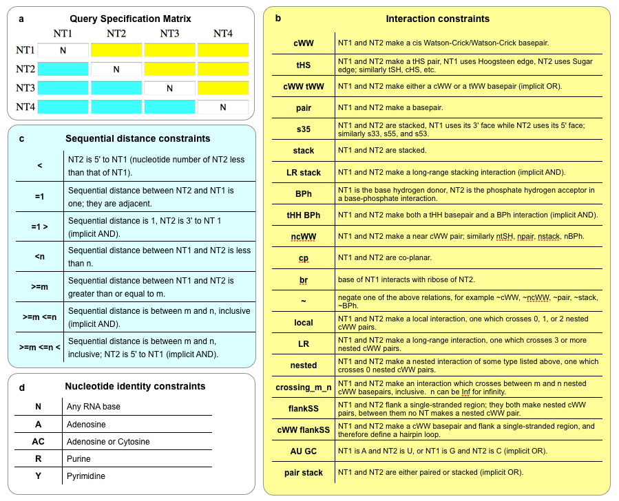
Nucleotides which border or delimit a single-stranded region
RNA hairpin loops occur at the end of a helix. In order to find them, it is useful to be able to search for the last canonical cWW basepair (AU, GC, or GU) before the hairpin. The two nucleotides in this basepair have two things going for them: they make a canonical cWW basepair and between them is a non-empty “single-stranded” part of the chain whose nucleotides make no additional nested canonical cWW basepairs. We say that these nucleotides border or delimit a single-stranded region. The following search finds such pairs:
clear Query % remove any previous Query parameters
Query.Name = 'cWW Border SS';
Query.Edges{1,2} = 'cWW borderSS';
Query.Diff{2,1} = '>';
Query.SearchFiles = {'1S72'};
oFR3DSearch
return
This search returns 72 instances from 1S72. What does that tell us about the structure? Why is it useful to put the > constraint between nucleotides 2 and 1?
Exercise: Symbolic search for hairpin loops and a little bit of context
The previous search only finds the flanking cWW basepair of hairpin loops, which does not tell us much about the structure of the hairpin. Let’s take a step in this direction by writing a search for the two nucleotides making the flanking cWW pair and the two nucleotides that are adjacent to those, inside the hairpin. Use the following diagram to design the search, making 1 and 4 be the cWW pair and satisfy the borderSS condition, and making nucleotide 2 have a higher nucleotide number than 1 but be adjacent in the chain, and making 3 have a lower nucleotide number than 4 but be adjacent in the chain. Don’t put any restriction on the number of nucleotides between 2 and 3.
Once you have the search designed, code it and run it with FR3D. Order the candidates by similarity. What lessons can you learn from these hairpins?
Exercise: Symbolic search for internal loops
Internal loops are more complicated than hairpin loops because they are made by two single-stranded regions and they have two closing canonical Watson-Crick basepairs. Draw a diagram for a 4-nucleotide query which will find all internal loops in 1S72 which have at least one nucleotide in each single-stranded region. Be sure to think about the cWW pairs, the borderSS relation, chain directionality, and anything else.

Type up this query and run it with FR3D. How many such internal loops are present in 1S72?
FR3D geometric and mixed searches
To this point, all of the searches we have done were made up of symbolic constraints, restrictions on basepairs and chain connectivity, to which we could add base stacking, base-backbone interactions using the different codes in the charts above. Now we turn our attention to geometric searches, where we start with a known instance and would like to find other instances of a similar motif. As we will see, one can add symbolic constraints to a geometric search in order to focus it and speed it up.
GNRA hairpin loop geometric search
There are a few common classes of hairpin loops in structured RNA molecules, and the GNRA loop is the most common. The string GNRA tells the “consensus” sequence of the hairpin, which is G followed by N (anything) followed by R (A or G) followed by A. Most instances of the GNRA fit this pattern, but certainly not all. Here are the parameters for a geometric search for GNRA hairpins in 1S72:
clear Query
Query.Name = 'GRNA hairpin geometric search';
Query.Filename = '1S72'; % file containing query instance
Query.NTList = {'804' '805' '806' '807' '808' '809'};
% nucleotide numbers of query
Query.ChainList = {'0' '0' '0' '0' '0' '0'};
% chains of query (optional)
Query.DiscCutoff = 0.5; % limit on geometric discrepancy
Query.Diff{2,1} = '>';
Query.Diff{3,2} = '>';
Query.Diff{4,3} = '>';
Query.Diff{5,4} = '>';
Query.Diff{6,5} = '>';
Query.ExcludeOverlap = 1; % exclude very similar candidates
Query.SearchFiles = {'1S72'};
oFR3DSearch
Let’s go through the lines which are new in this query. Query.Filename tells which PDB file contains the motif or fragment of interest, Query.NTList tells the nucleotide numbers, and because some PDB files contain multiple chains with overlapping nucleotide numbers, Query.ChainList tells the chain for each nucleotide. Query.DiscCutoff sets the maximum geometric discrepancy between a candidate and the query motif. Geometric discrepancy is somewhat like RMSD (root mean square deviation) and can be interpreted to have units of Angstroms. A discrepancy of 0.5 is a moderate number. Larger cutoff discrepancies will find more candidates but might take a long time to run. Query.ExcludeOverlap is a binary variable (0 or 1) which tells FR3D to exclude candidates which have many nucleotides in common, favoring the one having lower discrepancy with the query motif; 1 makes this happen, 0 tells FR3D not to bother.
Geometric discrepancy
The geometric discrepancy was defined in the 2008 paper FR3D: Finding Local and Composite Recurrent Structural Motifs in RNA 3D Structures, by Michael Sarver, Craig L. Zirbel, Jesse Stombaugh, Ali Mokdad, and Neocles B. Leontis, which is available at this link. It is a way of measuring how geometrically similar two sets of RNA nucleotides, provided that they have the same number of nucleotides. One gives two lists of RNA nucleotides, call them A1, A2, …, An, and B1, B2, …, Bn. Order is important, A1 is supposed to correspond to B1, A2 to B2, etc. It is important to allow for the possibility that A1 and B1 do not have the same base, so one needs to find a way to superimpose a G on a U, for example. The solution in the 2008 paper was to first calculate a geometric center of the heavy atoms for each of the n bases (see the figure below, taken from the 2008 paper) and find the rotation matrix which optimally rotates the centers of B1, B2, …, Bn onto the centers of A1, A2, …, An. The sum of the squares of the distances between corresponding centers is called the location error. After this superposition, the base in nucleotide A1 might not perfectly superimpose with the base in nucleotide B1, and so we calculate the angle (in radians) that would be needed to rotate one base to align with the other, using the standard orientations shown in the figure below. The sum of squares of the angles is called the orientation error. The discrepancy is then defined by  , where L2 is the location error and A2 is the orientation error. Dividing by n makes this a discrepancy per nucleotide, which has roughly the same meaning over a range of motif sizes.
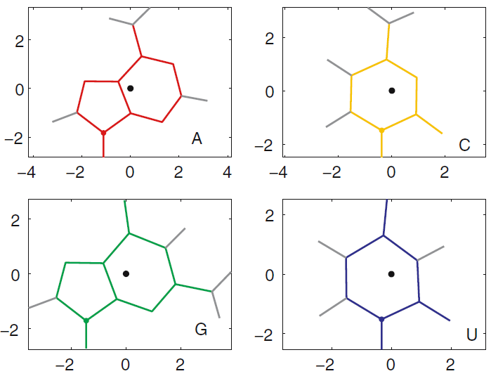
FR3D guaranteed results in geometric searches
An important characteristic of FR3D searches is that it is guaranteed to find all candidates whose geometric discrepancy with the query motif is less than or equal to the cutoff discrepancy, no matter what the chain connectivity is between the nucleotides in the candidate. In other words, a FR3D geometric search does not make any assumptions about the chain continuity of the nucleotides in the candidates, unless the user gives such constraints. In principle, if the query motif contains n nucleotides and we are searching in a structure having m nucleotides, there are roughly mn possible sets of n-nucleotide candidates, and none of them are excluded a priori. In practice, nucleotides that are more than 30 Angstroms apart cannot be in the same candidate, but that still leaves a large number of potential candidates to search through. The actual search procedure is described in the 2008 paper and is based on the fact that if A1, A2, …, An, and B1, B2, …, Bn are sets of nucleotides and Bi and Bj are much further apart than Ai and Aj are, then the geometric discrepancy between A1, A2, …, An, and B1, B2, …, Bn will be high, and we can be sure that B1, B2, …, Bn is not a good match to A1, A2, …, An, just by looking at those two nucleotides. Using pairwise distance checks, we can eliminate the vast majority of possible candidates and then calculate the full geometric discrepancy for those that are left, again rejecting those that are above the discrepancy cutoff.
Imposing pairwise symbolic constraints only serves to reject more candidates, and so speeds up the search. Generally speaking, any symbolic constraint that you can use which does not fundamentally constrain the search is a good one to use. Thus, for example, using the directionality constraints in the GNRA search above does not rule out any GNRA candidates, but does speed up the search quite a bit. On the other hand, if you remove those constraints, you find two new hairpins which are not unlike GNRA hairpins and which have a different chain connectivity order.
3-way junctions
Today we are going to use a FR3D search to find 3-way junctions, primarily in ribosomes, diagram their interactions, explore their conservation across bacteria, archaea, and eukaryotes, and look at the relative positions of their outgoing helices.
We begin by writing a FR3D search to find 3-way junctions with more than two nucleotides on each single strand. We are looking for six nucleotides that form the last Watson-Crick basepairs before the junction, and that also border the single stranded regions between the helices. The search should start like this:
clear Query % remove any previous Query parameters
Query.Name = 'Six flanking nucleotides of a 3-way junction';
Query.Edges{1,2} = 'cWW';
Query.Edges{2,3} = 'BorderSS';
Query.Diff{3,2} = '>';
Query.SearchFiles = {'Ribosome_list'};
oFR3DSearch
return
Your search should allow for all three symmetries of a 3-way junction, so that each instance is found 3 times. This will allow us to find junctions with similar geometries even though they occur with different strand orders.
Before running the search, please add the new yeast mitochondrial ribosomal large subunit 1VW3 to the file Ribosome_list in the folder FR3D/PDBFiles. We should be searching this structure whenever we search ribosomal structures. Also, you can download the Matlab binary file with all of the FR3D analysis of 1VW3 at this link (or update the Github FR3D repository on the dev branch). Save 1VW3.mat in FR3D/PrecomputedData. The circular diagram can be found at this link.
When I ran the FR3D search, it found 315 candidates. Please choose Sort by centrality and then, when it is done, Sort by centrality again. This will calculate geometric discrepancies between all 315 candidates. Then Quit navigation (to save the discrepancies) and oDisplay to start the display again. Now choose Order by Similarity. Figure 99 will show you a few clusters, the largest of which seems to be repeated 3 times. This is because each 3-way junction appears three times in the search results, but the three appearances do not superimpose on one another. Choose Order by Similarity again to select just one instance of each 3-way junction in a way that preserves the clusters.
Focus on the largest cluster by choosing Navigate with Figure 99 and then clicking on the upper right hand corner of the cluster. This will mark those candidates, then choose Display marked only. Below is the heat map of mutual discrepancies that I get when I do this search. Let’s focus on the candidates in the lower right corner, since they are most geometrically similar.
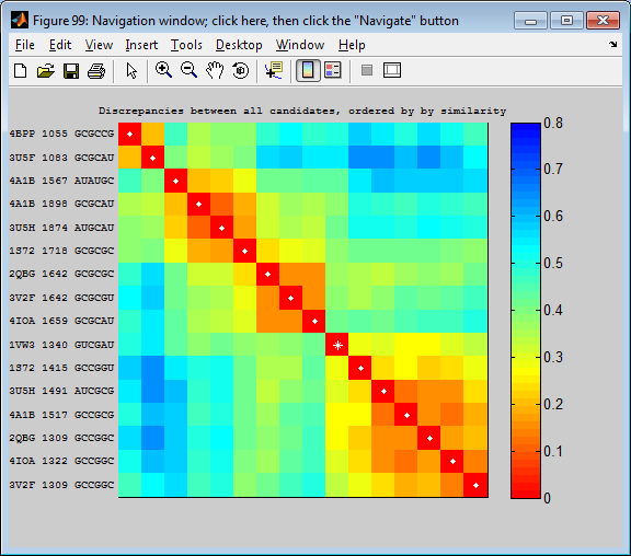
Here you see candidates from the following structures:
- 1VW3 - yeast mitochondrial large ribosomal subunit (eukaryotic mitochondria)
- 1S72 - Haloarcula marismortui large ribosomal subunit (archaea)
- 3U5H - yeast large ribosomal subunit (eukarya)
- 4A1B - Tetrahymena thermophila large ribosomal subunit (eukarya)
- 2QBG - E. coli large ribosomal subunit (bacteria)
- 4IOA - Deinococcus radiodurans large ribosomal subunit (bacteria)
- 3V2F - Thermus thermophilus large ribosomal subunit (bacteria)
Amazingly, there is one candidate from each of the large ribosomal subunit classes that have been solved to near atomic resolution (the 1VW3 structure is done by cryo electron microscopy).
Open the circular diagrams for each of these structures. These are found in the FR3D/CircularDiagrams folder from the large zip file that I provided at this link. Check to see if these 7 instances occur in the same place in the secondary structure, so that we can figure they are homologous (have a common ancestor, long, long ago).
For reference, here are the main ribosomal small subunit structures as of June 29, 2014:
- 2AW7 - E. coli small ribosomal subunit (bacteria)
- 1FJG - Thermus thermophilus small ribosomal subunit (bacteria)
- 3U5F - yeast small ribosomal subunit (eukarya)
- 4BPP - Tetrahymena thermophila small ribosomal subunit (eukarya)
Now start to diagram these 3-way junctions. Please arrange the nucleotides in clockwise order, starting with the longest strand with nucleotides listed vertically from bottom to top, on the left of the diagram. Start with a bacterium, then the mitochondrion, then the archaeon, then a eukaryote. If you draw the diagrams in the same way, it will make it easier to see similarities between the structures.
The next cluster with similar geometry has 3 instances from bacteria, right in the center of the heat map above. Choose one of those and diagram it in the same orientation as the ones you have just done. Also check to see where this 3-way junction is in the circular diagram.
What determines the 3D structure of a 3-way junction?
Let’s continue with the large cluster of 7 instances of a 3-way junction from the previous class period. Ask these questions about the instances:
- Does the junction have similar internal structure across different homologues? Does it have conserved basepairs, conserved stacking, conserved base-backbone interactions? If so, these are indications that the internal structure of the junction is important to determine its 3D structure.
- Look at the helices joined together by the junction. In some junctions, two of the helices are stacked on one another, so that they appear to form one continuous double helix whose geometry is almost undisturbed by the third helix sticking out to the side. Is this the case with this cluster?
- In other junctions, two of the helices sit side by side, like crayons in a box. This allows additional interactions between the helices to help stabilize the geometry of the junction. Does this happen?
- In other junctions, there are different long-range interactions between the stems radiating from the junction, like pseudoknots or A-minor interactions (where one, two, or more adenines make basepairs with the sugar edges of the G and C in a Watson-Crick basepair). Does this happen here?
So far, we have been studying the largest cluster of 3-way junctions in a search that returned 315 instances. Let’s look at the other clusters and divide and conquer: each person choose one of the clusters and address the four questions above.
The previous search found 3-way junctions in which there are 3 flanking Watson-Crick basepairs and 3 single-stranded regions. The way the BorderSS relation is coded in FR3D, the single-stranded regions must have at least one nucleotide between the nucleotides making Watson-Crick basepairs. However, some junctions have one “empty” single-stranded region. Adjust the search above to find such junctions by using one constraint like this:
% Query.Edges{2,3} = ''; % no constraint on interaction between 2 and 3
Query.Diff{3,2} = '> =1'; % sequentially adjacent nucleotides
Note that you only need one constraint like this. There are 39 such 3-way junctions in the ribosome list. In many cases, you will find that bases 2 and 3 are stacked on each other, but not in all cases. Download the FR3D search results for the whole non-redundant list at this link.
Internal loop sequences with different geometry
Today we will start the class by looking at instances of internal loops that have the same sequence but different geometry. The instances can be viewed at this link. We will look at a few examples together, then I would like you to each take a block of instances and decide whether they all have substantially the same geometry or whether one of them differs in a significant way, especially when they make different basepairs.
Exercise
The phrase “one sequence, one structure” is appealing for RNA because it would mean that once you know the sequence of an RNA, there is a unique secondary or 3D structure associated with it. We know that this isn’t strictly true, because we know about riboswitches that change their secondary and 3D structure when a ligand binds. On the other hand, with Watson-Crick complementary sequences, we pretty well expect that “one sequence, one structure” will hold. What about other small structural units like internal loops? If “one sequence, one structure” holds, then we ought to be able to predict the 3D structure of these units fairly accurately. In some cases, this assumption seems to be justified, but in others, one sequence can have a variety of 3D structures.
I have collected together many instances of internal loops from the RNA 3D Motif Atlas on this web page: http://rna.bgsu.edu/experiments/jsmol/IL_with_identical_sequences.htm They are organized into sets which have the same “interior” sequence (the bases between the flanking Watson-Crick pairs). Within each set, they are ordered so that sequences with the same flanking bases are near each other. Each line tells the sequence of the internal loop, the loop ID, the motif group that it comes from in the RNA 3D Motif Atlas, and the base and nucleotide number of one instance in the loop. Notice that in the first 870 instances, there are always at least two motif groups listed, which suggests that these instances may have different geometries. I have added annotations to the first several sets to describe the differences in geometry. Please read those and look at a few of the instances to learn how I’ve annotated them.
The assignment is for you to annotate other sets of internal loop instances in the same way. You can print out lines of text and write your annotations on paper or, better yet, view the page source, copy it into an editor, and add your annotations to the end of each line as I have done. Then I can paste your annotations into the source of the web page and make this a useful resource. Neocles Leontis is pretty excited about writing a paper about these examples. If you are interested in working on a paper like this, let me know.
Here are things to look for.
- Do all of the instances have essentially the same geometry even though some of them are in different motif groups? That can happen, and I’ve moved such sets to the bottom of the page when I found them. If you think this is happening, add that as an annotation. But be careful. The set from 448 to 475 looked the same to me until I looked closer and saw that the instances from IL_82444.1 have a GG cWH basepair instead of cWW. In such a small motif, that is a big difference.
- Do some of the instances have bases bulged out of the motif (and interacting with other RNA or protein), while some of the instances have no bulged bases? This is a very common thing and goes by the name induced fit which means that the external context of a loop influences the geometry of the loop. This seems to happen more often with A’s, especially when there are multiple A’s in a row.
- Something of a Holy Grail would be to find two instances with different geometries but no obvious induced fit that is causing it. This would suggest that some motifs have two competing stable geometries. Seek the Grail!
Rustbelt RNA 2018 workshop
This workshop will entail short, informative lectures on basic principles of RNA structure, interactions, and
structural motifs, interspersed with hands‐on visualization and analysis of RNA 3D structures, using free software and online databases. Participants will learn how to find high quality 3D structures for RNA molecules of interest using resources we have developed in partnership with the Nucleic Acid Database (NDB). We will provide tutorial guidance in the use of 3D viewers like Swiss PDB Viewer to view and analyze RNA and RNA‐protein 3D structures. Participants will be introduced to recurrent interactions in RNA 3D structures (basepairs, base stacking, base‐backbone, and RNA‐protein interactions) and how to obtain annotations of these interactions for any RNA structure in PDB/NDB. We will discuss the constraints that these interactions put on sequence variability, and how to use those constraints to design experiments to investigate hypothesized interactions or to design RNAs with desired 3D structures.
Enumerating Basepairs using Triangle Bases
Getting and using the Swiss PDB Viewer Program: Short Presentation
Instructions for PC
Start at https://spdbv.vital-it.ch/disclaim.html On the next page, click the link for Microsoft Windows. This downloads a .zip file. Extract, then move the folder SPDBV_4.10_PC to a folder on your computer for programs. Inside the folder, double click spdbv.exe to run the program. Close the "thanks" window, then use the menu to open a PDB file.
Instructions for Mac
Start at this link: ftp://ftp.vital-it.ch/tools/SPDBV/ . For those using OSX 10.11 (El Capitan) and earlier versions, click on SPDV_4.1.0_OSX.zip to download it while those using OSX 10.12 (Sierra) or higher should click on SPDV_4.1.1_OSX.zip to download it. Once the download is complete, double-click on the file to unzip it and then move the folder SPDBV_4.1.0_OSX or SPDBV_4.1.1_OSX to your application folder (where you put programs!). Inside the Application folder, double click the Swiss-PdbViewer icon to run the program:
Users of OSX 10.12/10.13 might see the following error (rotolib.aa error) when they try to open Swiss PDB-viewer. Follow the instructions in this page to resolve the problem: https://kb.unca.edu/help/how-to-articles/swiss-pdb-viewer
PDB file to open to test SwissPDB viewer: We have colored the helices in the tRNA in PDB file 1EHZ, available at this link.
Sample tRNA PDB file to download at this link.
Goals of the Rustbelt Workshop
- Methylation of RNA bases in tRNA - relation to structure
- Specificity of A-riboswitch (PDB file 1Y26) vs. G-riboswitch (PDB file 1Y27). Both have U on the Sugar-edge but Differ in the pairing on the Watson-Crick (WC) edge. (See below)
- 3SKI is deoxy-G riboswitch. Has a C on the Sugar-edge instead of U! Question: Why?
- CRISPR: - RNA-DNA hybrids that are cut in the DNA strand
- RNase H: An enzyme that cuts the RNA only when it is in an RNA-DNA double-helical hybrid
- G-stabilized interactions: G makes more H-bonds than any other Base and so forms some of the most favorable (lowest energy) interactions, some of which are G-specific and others G-favored.
- Base-specific Interactions: Each of the other bases, (A, C, and U) also forms some specific interaction.
- Isosteric interactions: Many interactions can be formed by different combinations of bases, resulting in geometrically identical (but not chemically identical) - “Iso-steric” = “same-space occupying” interactions.
- Examples from tRNA-mRNA decoding - at each of the three codon positions. How Redundancy of the genetic code works. Relation to tRNA modification.
- RNA-protein interactions
- RNA riboswitch that distinguish G from A or C from U
- A-minor interactions using As in the ribosome to ensure that cognate tRNA is bound to mRNA Codon in A-site.
- Error-checking in RNA polymerase, and DNA replicase. But this has to use Protein.